Grid creation

Checklist

• make sure that electrodes are separated by at least one node

• make sure that the electrodes are separated from the border by a few nodes

• check the boundary conditions

• check the coarseness of your grid (coarse for the first inversions, fine for presentation; if the grid is very large use fine cells near the electrodes and coarse cells near the boundaries)

Regular grids

At this point the CRTomo-tools do not provide a tool to generate regular grids.

There is an old grid generator available (Griev) - however compilation and usage has not been tested recently.

Irregular grids

The command to create irregular grids is:

$ cr_trig_create

You need to create the files described down below first (required files: electrodes.dat, boundaries.dat) to give the program the information about the grid it shall create. Use the -h command to see the possible options.

The program will create a subdirectory with a unique name and store the final grid files (and all intermediate files) in there. The output directory is given in the last line of output.

Alternatively, an output directory can be provided as the first parameter:

$ cr_trig_create [output_directory]

At least one node should separate two electrodes. One way to ensure this is to set the characteristic length to about half the minimal electrode distance in the grid. You can specify the characteristic length in the char_length.dat.

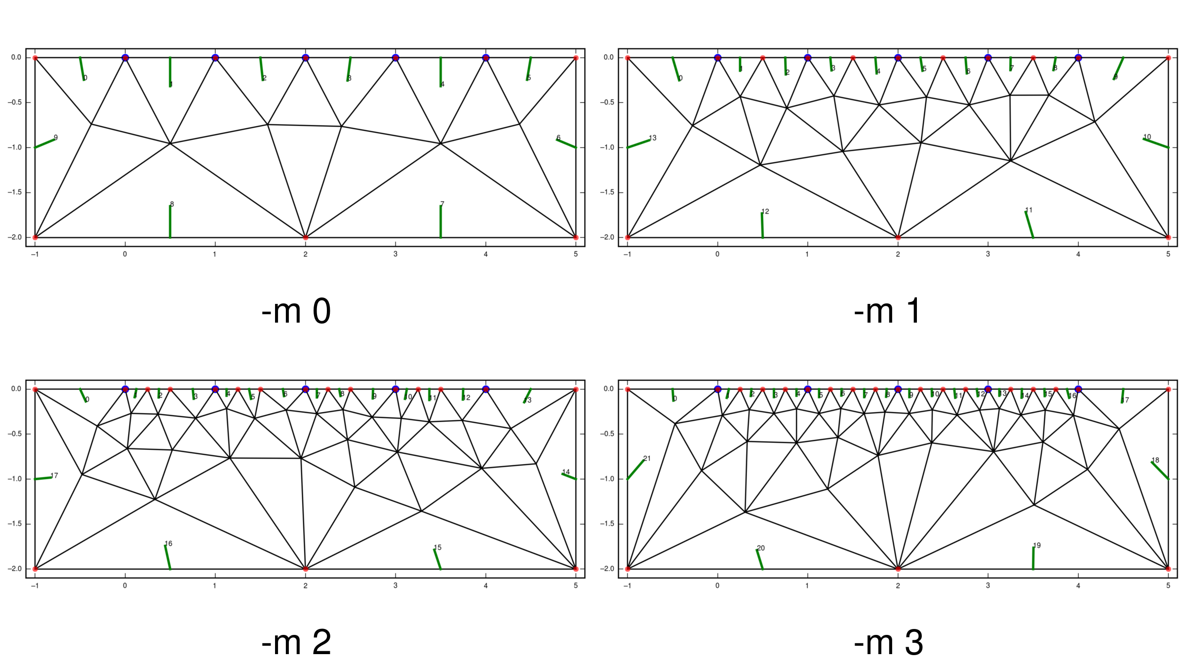
Another one is to use the -m switch, which ensures that at least the given number of nodes separates successive electrodes. This works only for grids with surface electrodes. Otherwise it is not clear which nodes lie between any two electrodes. Also, the algorithm does not add nodes before and after the first and last electrodes, respectively. Therefore, make sure to add enough boundary nodes at the grid edges to prevent large modelling errors. You specify you boundaries in the boundaries.dat.

Due to the simple nature of the algorithm, only odd numbers should be used for -m. Even numbers usually result in non-equidistant nodes.

Below the final grids generated by the following commands are shown:

$ echo 4 > char_length.dat
$ cr_trig_create -m 0 grid_m0
$ cr_trig_create -m 1 grid_m1
$ cr_trig_create -m 2 grid_m2
$ cr_trig_create -m 3 grid_m3

Best practices

• check the output for red warnings from GMSH. This is always an indicator for a non-functional grid.

• at the end of the grid creation CutMcK is called to create an optimal node arrangement within the grid. Check this output for the string

  zero nodes found
  

  This also is an indicator for problems.

• Use an electrode characteristic length of half the minimal electrode distance. This ensures that at least two elements are located between any two electrodes. Use the boundary characteristic length (larger values) to increase the element size far away from the electrodes.

  Alternatively, use the -m switch to add additional nodes between the electrodes.

• a plot of the grid is created in the output directory, check it.

• use Griev (or some other grid viewer) to inspect the grid, especially at the electrodes.

• grid cells should not have steep angles, as this decreases the FE solution quality.

• make sure that no electrodes are located on any edge nodes of the grid. This drastically reduces modelling accuracy.

• for circular grids, the following code snippet can be of help:

  #!/usr/bin/python
  # -*- coding: utf-8 -*-
  """
  Created on Tue Apr 21 15:26:22 2015
  
  @author: stamm, mweigand
  """
  import math
  import numpy as np
  
  
  def get_points(R, points):
      p = []
  
      n = int(points)
      for i in reversed(range(0, n)):
          phi = 2 * np.pi / n * i
          x = R * math.cos(phi)
          y = R * math.sin(phi)
          p.append((x, y))
          # print("%4.4f \t %4.4f" % (x, y))
      return p
  
  if __name__ == '__main__':
      # radius = raw_input("Bitte Radius aingeben: ")
      # R = float(radius)
      R = 0.4  # [m]
      electrodes = get_points(R, 24)
      boundaries = [x + (12, ) for x in get_points(R, 48)]
  
      np.savetxt('electrodes.dat', np.array(electrodes))
      np.savetxt('boundaries.dat', np.array(boundaries))
  

electrodes.dat

(X,Y) coordinates of all electrodes. Each electrode in one line:

24.0000 -34.0000
24.0000 -35.0000
24.0000 -36.0000

The line number corresponds to the electrode number in the final grid.

Warning

The -m switch can only work if the electrodes are arranged in successive order, i.e. either clockwise or counterclockwise. If other electrode arrangements are used, add all required nodes directly to boundaries.dat (position must be computed by other means, in this case).

boundaries.dat

(X,Y) coordinates of the nodes comprising the boundaries of the grid. If electrodes lie on the surface, also specify them in the boundaries.dat file. Doublets will be automatically removed.

Note

Specify the boundary elements clockwise! Anything else will lead to problems, either in the grid generation, or the modelling/inversion runs.

The third column denotes the boundary element type of the boundary described by the node and the next node. The last node denotes the boundary type of the element from the last to the first node.

-1.0000 1.7700  12
1.0000 1.7100   12
3.0000 1.5100   12
5.0000 1.4300   12

Note

Make sure to first write down the number 12 (neumann) boundaries, and then the number 11 (mixed) boundaries. This should prevent most problems with the grids.

char_length.dat (optional)

The file is expected to have either 1 or 4 entries/lines with characteristic lengths > 0 (floats). If only one value is encountered, it is used for all four entities. If four values are encountered, they are assigned, in order, to:

1. electrode nodes

2. boundary nodes

3. nodes from extra lines

4. nodes from extra nodes

Note that in case one node belongs to multiple entities, the smallest characteristic length will be used.

If four values are used and the electrode length is negative, then the electrode positions will be read in (todo: we open the electrode.dat file two times here…) and the minimal distance between all electrodes will be multiplied by the absolute value of the imported value, and used as the characteristic length:

\[l_{electrodes} = min(pdist(electrodes)) * |l_{electrodes}^{from file}|\]

The function scipy.spatial.distance.pdist is used to compute the global minimum distance between any two electrodes.

It is advisable to only use values in the range [-1, 0) for the automatic char length option.

The characteristic length is the desired element size around a given node. However, if the distance between two nodes is smaller than the characteristic length, then this distances determines the given element cell. This behavior has the consequence that large characteristic lengths can lead to inhomogeneous cell sizes, and therefore reduce to overall-element number. Elements clustered around the nodes will then still have an acceptable size.

Default value is 1.

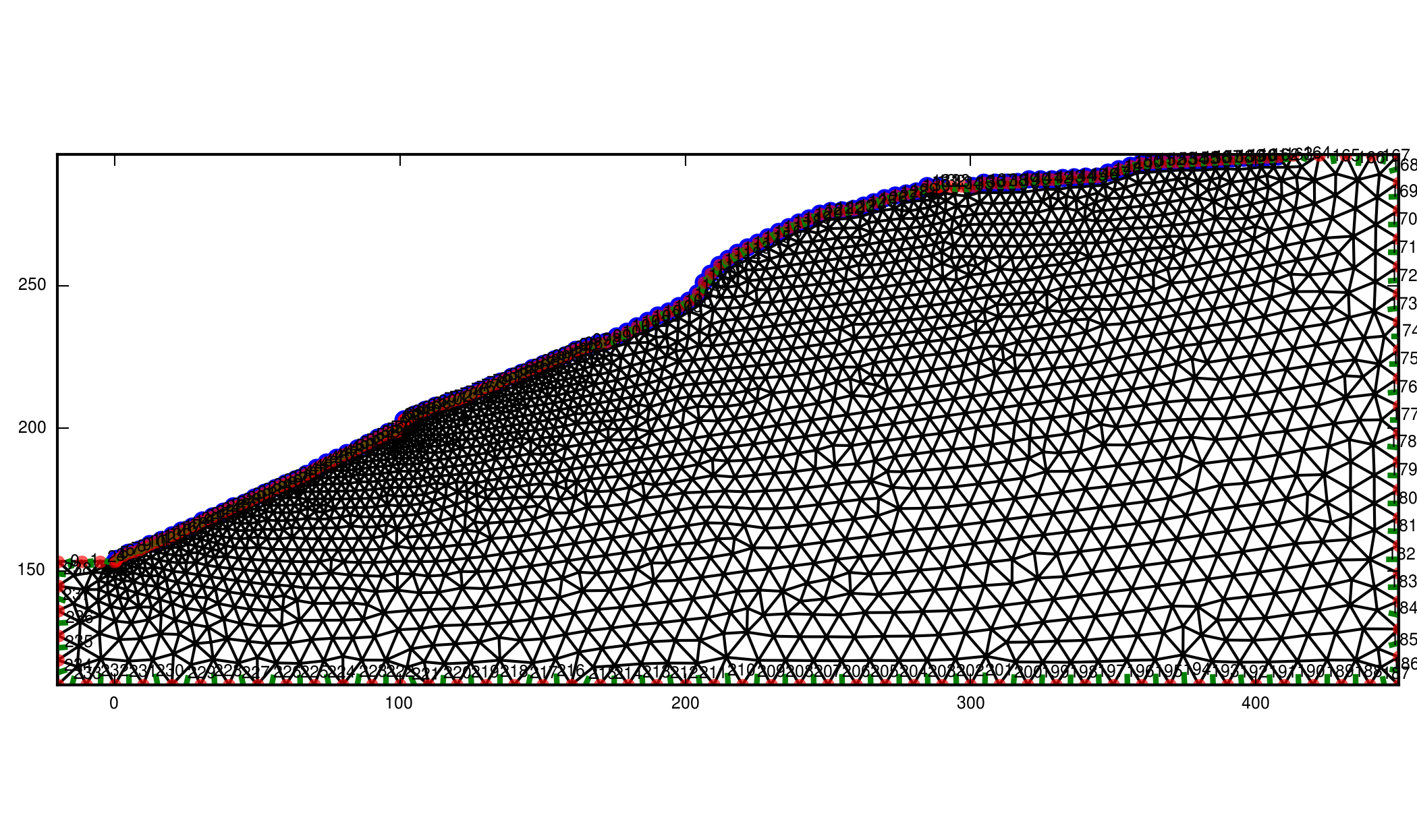
In the following example you see the char_length.dat and the created grid. Note that the cells are coarser at the boarders but still fine at the electrodes. This is usefull, when using such a big grid.

5.0
10.0
5.0
5.0

extra_lines.dat (optional)

Extra lines (i.e. to model layer interfaces or water levels) can be included in the grid using the file extra_lines.dat. Each line holds the start (x1,y1) and end (x2,y2) point of this line.

x1 y1 x2 y2
0.0 -10.0 26.0 -10.0

Start/end points lying on the boundaries must be included in the boundaries.dat file.

extra_nodes.dat (optional)

Extra nodes to be included in the grid (e.g. to refine the mesh at certain positions) can be specified in this file, one point (x, y) per line:

0.0 0.0
10.0 -26.0

Extra points that lie on the boundaries of the mesh must be included into the boundary.dat file!

Note

Be careful with placing extra nodes in the vicinity of boundaries. This can easily lead to errors in the grid generation. Sometimes it helps to add a few more nodes in the direct vicinity of this one node.

Note

In the vicinity of boundaries, or other constraining elements, the characteristic length can play an important role in preventing a successful grid generation. If the characteristic length is too large, elements cannot be created that include the extra nodes. Try reducing the char. length in those cases.

gmsh_commands.dat (optional)

If this file exists, the content will be appended to the commands.geo file used to create the grid (i.e. GMSH commands should be used).

Introducing structures into a mesh using Inkscape

Sometimes, it can be useful to adapt the grid to certain geometries or structures (e.g., interfaces, anomalies with certain shapes, etc…). Furthermore, turning off the regularization along certain interfaces can allow for sharper contrasts at desired boundaries. For this, additional nodes can be included using svg files. Here, we show how both of these goals can be achieved via manipulation of the mesh using Inkscape.

Exemplary workflow:

• Create a triangular mesh using cr_trig_create (i.e., using electrodes.dat, boundaries.dat, and char_length.dat)

• Run grid_convert_boundary_to_svg to generate an svg file containing the mesh boundaries (the file is called out.svg)

• Open the svg file in Inkscape

  • Add layers with one of the following naming schemes:

    • constraint_*

    • special_*

    • ???

• For example: constraint_1

  

• Add straight lines (SHIFT+F6) and define boundaries and regions (for region, close the polygon). It is not important to close the polygons if you just want to add interfaces for regularization decoupling. However, in order to modify forward models, it is advisable to close polygons (i.e., the last line should end on the starting point of the first one).

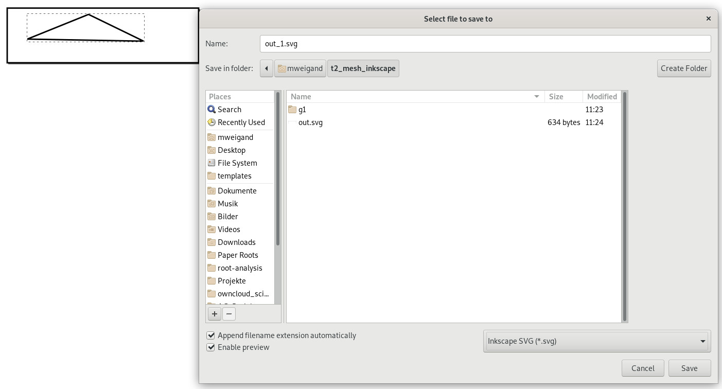
• Save the file to out_modified2.svg as type Inkscape svg

  

• Run grid_parse_svg_to_files out_modified2.svg. This command should rename your original boundaries.dat to boundaries_orig.dat and generate a new one that incorporates any (required) structure on the boundaries.

  The command will also generate two files for each layer defined in the svg file:

  • A file [LAYER_NAME].dat :

  • A file mdl_[LAYER_NAME].dat :

• Create extra_lines.dat:

  cat contraints_1.dat > extra_lines.dat

• Regenerate the mesh:

  cr_trig_create grid_with_constraints

• See the corresponding example in “Examples: Grid handling”

Further Reading:

• Check and sort boundary polygon:

  • http://stackoverflow.com/questions/13935324/sorting-clockwise-polygon-points-in-matlab

  • http://stackoverflow.com/questions/1165647/how-to-determine-if-a-list-of-polygon-points-are-in-clockwise-order

• for an explanation of the characteristic length, see:

  • http://geuz.org/gmsh/doc/texinfo/gmsh.html#Mesh