Basics

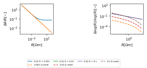
In the inv.ctr file the mag RMS is computed using only the magnitude error, while the phase RMS is computed only with the phase error. The data RMS uses the complex error composed of the square root of the sum of squares of magnitude and phase errors.

Usage Aspects

Artificial Noise

The file crt.noisemod looks like follows:

1          # Ensemble seed
5.00       # Relative error resistance A (noise) [%] von dR=AR+B
0.100E-03  # Absolute error resistance B (noise) [Ohm m]
0.00       # Phase error parameter A1 (noise) [mRad/Ohm/m] von dp=A1*R^B1+A2*p+p0
0.00       # Phase error parameter B1 (noise) []
0.00       # Relative phase error A2 (noise) [%]
0.500      # Absolute phase error p0 (noise) [mRad]

The file will be created by CRTomo even when the noise levels are coupled to the error model, and filled with the actually used parameters.

CRTomo creates the files inv.mynoise_rho, inv.mynoise_pha and inv.mynoise_voltages in its execution directory when noise is added to the measurements. Those files contain the absolute noise levels added to the data, and the resulting data used in the inversion.

Error estimates

(Source code, png, hires.png, pdf)

Error ellipsis

For the master branch:

Complex	FPI	Error ellipsis in complex inversion
X	X	–
X	–	X
– (DC)	–	X

Cuthill-McKee Algorithm

The ordering of the nodes in the elem.dat file can be changed to reduce the amount of computing power needed for forward modellings and inversion runs (The bandwidth of the stiffness matrix \(S\) is reduced).

While the order of the nodes will be changed, the order of elements will not be changed. You cannot use a non-CutMcK’ed elec.dat with an optimized elem.dat file, as the electrodes are assigned to node numbers which were renumbered.

The CutMcK algorithm we use doesn’t change the coordinates. It merely renumbers those coordinates. To find the coordinates of the element nodes, for each node \(n_i\) of the element follow the steps:

• 1. Go to the \(n_i\)-th node of the elem.dat file.

• 2. The index of the coordinates are specified by the number located in the first column.

Example: Suppose you have the element nodes:

99 100 101 102

and the snippet from the elem.dat file (the numbers in () indicate the number of the nodes corresponding to the line number + 4 lines for the header):

...
( 99)   205 3 4
(100)   304 5 3
(101)   405 1 2
(102)   604 0 9
...
(205)   321 0 0
...
(304)   221 0 -1
...
(405)   665 1 -1
...
(604)   123 1 0

For the first node specified for the element (node 99), go to line 99 and find the index for the coordinates (205). Thus the coordinates for this node are \((0,0)\). The other coordinates resolve to \((0,-1)\), \((1,-1)\), and \((1,0)\), respectively.

Sort the nodes

If you want to sort the nodes so that the node indices in the element definitions point directly to the correct coordinates, do the following:

For each line (node):

1. Find the line (node) where the first column holds the number for the current node.

2. Move the coordinates of the current node to this position.

Warning

The sorting cannot be done in only one array!

\(\lambda\) value

There are three ways to calculate the initial value for \(\lambda\):

1. Citation from Kemna, 2000: “Following a suggestion of Newman et al, 1997, an adequate starting value \(\lambda_0\) at the first iteration step may be estimated from the row sums of the matrix product \(A^H W_d^H W_d A\). Such a choice properly scales the regularizing term \(\lambda W_m^T W_m\) in eq. (3.53) at the beginning of the inversion process. However, whereas Newman et al., 1997 use the maximum absolute row value which occurs, for the problem considered herein five times the corresponding mean value has been found to be sufficiently large. Taking in addition the smoothing parameters \(\alpha_x\) and \(\alpha_z\) into account, it is:

\[\lambda_0 = \frac{2}{\alpha_x+\alpha_z} \frac{5}{M} \sum_{m=1}^M \left| \sum_{j=1}^M \sum_{i=1}^N \frac{{\overline{a}}_{im}a_{ij}}{{\overline{\epsilon}}_i\epsilon_j}\right|,\]

where \(\overline{\; }\) denotes complex conjugation.”

2. Easylam: \(\lambda_0\) = Number of model cells

3. User supplied lambda_0

Roland Martin (Juli 2012):

Dann noch etwas zur generellen Vorgehensweise mit der Lambda Bestimmung:

Ich hatte seinerzeit mal aus Zeit-Kosten-Gründen für (nz=Anzahl der Gitterpunkte in z-Richtung) den switch eingebaut für eine “einfache” \(\lambda_0\) Bestimmung (taking easy lam0). Das ist eine mehr oder weniger brauchbare Einstellung, die man nicht immer nutzen sollte, sondern nur dann, wenn man sich sicher ist, was man tut.

Mein Vorschlag für ein Vorgehen ist folgendermaßen:

Bei einem ersten Inversionslauf nimmt man für diesen switch (nz) nz=0, dann wird das \(\lambda\) “ordentlich” bestimmt, also:

\(\lambda_0 = \sum (WJTWJ_{ii})\)

Wenn der Wert in etwa der Anzahl der Modellparameter (oder auch Messungen, je nach dem) entspricht, dann kann man in den darauf folgenden Inversionsläufen entweder \(nz=-1\) wählen (dann wird MAX(m,n) als Startwert gesetzt), oder man notiert sich den Wert aus dem ersten Lauf und gibt diesen dann als Integer mit einem Minus davor an, also \(nz = -< \lambda_0\) vom ersten Lauf.

Wenn man nz=-1 immer nimmt, ohne das vorher zu prüfen, dann sucht man evtl nicht in die richtige Richtung, denn CRTomo braucht im Grunde einen maximalen Startwert für die lambda suche, keinen mittendrin oder sogar ganz unten (im Sinne der Anpassung), denn es benutzt ein Such-Verfahren, welches am liebsten einen Startpunkt außerhalb und oberhalb des Minimums hat. Unterhalb (lambda zu klein) ginge theoretisch zwar auch, ist aber insofern schlecht, da hier der singuläre Charakter von JTJ, bzw der Sensitivitätsmatrix viel stärker zum Tragen kommt, als wenn man mit einer starken Dämpfung (=großes Lambda) anfängt. Die Ergebnisse sind dann also in der Regel “schrott”.

For normal use the first method should always be used! If you know what you are doing, easylam0 can be used. But be carefull: If the initial value of methods 2 and 3 is too small, it is unlikely that CRTomo can recover and the results will be suboptimal.

Roughness

Cited from Kemna et al 2000: “A measure of the model roughness is introduced by \(\Psi_m (m) = \iint ||\nabla m||^2 dxdz,\) where \(||\;||\) represents the standard \(L_2\)-norm, and \(\nabla\) is the 2D gradient operator.”

Stepsize

Cited from Kemna et al 2000: “There (…) exists (an) approach to minimize nonquadratic functions like \(\Psi\) by the CG (Conjugate Gradient) technique alone, going back to (Polak et al.,1969). Herein, at each CG relaxation step the model itself is updated, i.e., \(m_{k+1} = m_k +\alpha_k p_k\) [cf. the corresponding line in the algorithm (3.55)], where the step length \(\alpha_k\) is chosen to minimize \(\Psi\) as a function of \(\alpha_k\), i.e., a line search is performed. The new gradient of \(\Psi(m_{k+1})\) is directly evaluated and used to determine the subsequent CG diretion \(p_{k+1}\). Thus, this approach involves only a single iteration cycle (the outer Gauss-Newton iteration vanishes) at the price of having to calculate the gradient vector, virtually given by eq (3.54), at each CG step (note that the Hessian is not exploited at all). The connection between the combined Gauss-Newton/CG method and the Polak-Ribière method is dicussed in Hestenes et al.,1980.

Steplength

The steplength \(s\) scales the model update in each iteration:

\(m_{q+1} = m_q + s \Delta m_q ,\)

where \(s \in [0,1]\). This scaling, also called steplength damping, is used to prevent the solution to over shoot the best solution due to the non-linearity of the underlying problem.

Difference inversion

Note

Difference inversion is only available for DC data!

• voltages of all involved data files must be the same for all lines

Required input:

• full, absolute inversion of time0:

  • volt.dat file for time 0: volt0.dat

  • model response of time0 inversion, volt0X.dat

  • inversion model for time0: rho0X.mag

crtomo.cfg snippet (with preceding line numbers):

4 ../mod/volt1.dat
5 ../inv
6 T ! difference inversion?
7 ../../time0/mod/volt.dat
8 ../../time0/inv/rho05.mag
9 ../../time0/inv/volt05.dat
10 iseed variance
11 0    ! # cells in x-direction
12 -1   ! # cells in z-direction

Changes to output files:

rho0X.mag:

3828       2.7374096866950728
-1.6500     -0.1500      1.9428     -1.9318     -1.7267      1.9698      0.2204
-1.3500     -0.1500      1.9408     -1.2176     -1.0756      1.2326      0.1395
-1.0500     -0.1500      1.9370      0.3139      0.2707     -0.3129     -0.0363
-0.7500     -0.1500      1.9316      2.6170      2.1785     -2.5503     -0.3064
...

Columns for lines 2-:

line	plot-index	can use –cmaglin	description
	0		center of element, x coordinate
	1		center of element, z coordinate
	2	yes	inversion result, absolute resistivity (log10-values), rho
	3	yes	starting model (log10, resisitivity), rho0
	4	yes	log10(rho) - log10(rho0)
	5	no	(rho - rho0) / rho0 * 100
	6	no	(sigma - sigma0) / sigma0 * 100

The additional columns 4-7 can be plotted using the –column switch of plot_td.py:

# starting model log10
plot_ty.py --column 3
# starting model linear
plot_ty.py --column 3 --cmaglin
# log10(rho) - log10(rho0)
plot_ty.py --column 4
# rho/rho0
plot_ty.py --column 4 --cmaglin
# (rho - rho0) / rho0 * 100
plot_ty.py --column 5
# (sigma - sigma0) / sigma0 * 100
plot_ty.py --column 6

Error parameters must be adapted according to the new data parameterization of the difference inversion.

Regularization

Calculation of K-factors

The K-factors are calculated in the module bkfak.f90. The resulting variable kfak(i) includes the K-factor for each electrode configuration i of a measurement.

Method of image charges

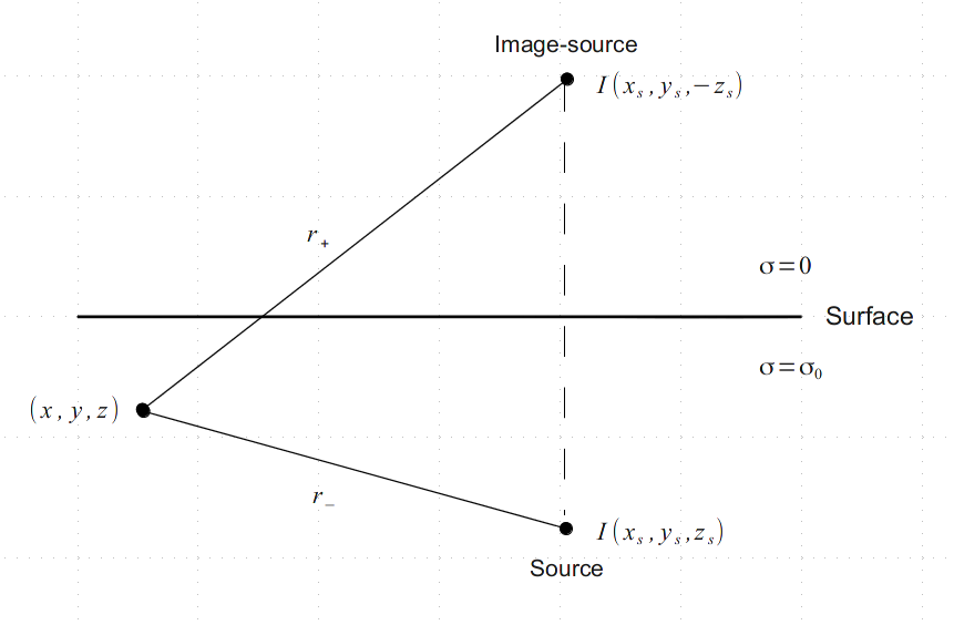
In order to determine the potential at any point in space due to a quadripole (whether you have no surface array) you have to use the method of image charges. So the charge within the surface, for example (0,0,-z), will produce the same electrical field as a mirror charge located in (0,0,z). This satisfies the boundary condition, that the potential along the surface must be zero.

The potential in full-space is formulated as \(\varphi(r) = \frac{I}{4\pi\sigma_0 r}\). Hence the potential of one borehole-electrode can be described by the principle of superposition:

\(\varphi(x,y,z) = \frac{I}{4\pi\sigma_0 r} \left(\frac{1}{r_{-}} + \frac{1}{r_{+}}\right)\), with

\(r_{-}^{2} = (x-x_s)^2 + (y-y_s)^2 + (z-z_s)^2\) and

\(r_{+}^{2} = (x-x_s)^2 + (y-y_s)^2 + (z+z_s)^2\).

Note

If \(z_s = 0\) then \(r_-\) equals \(r_+\) and you will receive a solution for a half-space.

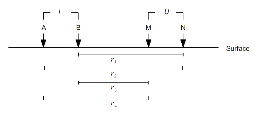
Typically you don’t want to measure the potential at one point but the potential-difference between two points (one current and one voltage electrode). The four possibilities for a quadripole arrangement are:

• \(r_1\) (Between B and N)

• \(r_2\) (Between A and N)

• \(r_3\) (Between B and M)

• \(r_4\) (Between A and M)

The value for the apparent resistivity of one quadripole can be calculated with \(\rho_0 = \frac{1}{\sigma_0} = K \cdot \frac{U}{I}\) with

\(K = \frac{4\pi}{\frac{1}{r_1}-\frac{1}{r_2}-\frac{1}{r_3}+\frac{1}{r_4}}\).

Each \(r\) is calculated by the method of image charges with \(r = r_{-} + r_{+}\).

Guidance through bkfak.f90

Declaration of variables and open file tmp.kfak.

pi = dacos(-1d0)
xk = 0D0
yk = 0D0
CALL get_unit(fp)
OPEN (fp,FILE='tmp.kfak',STATUS='replace')

Starting loop over all measurements, where nanz is the number of measurements, coming from datmod.f90.

do i=1,nanz

Reading in current and voltage electrodes with variables strnr and vnr declared in datmod.f90 and convert them.

elec1 = mod(strnr(i),10000)
elec2 = (strnr(i)-elec1)/10000
elec3 = mod(vnr(i),10000)
elec4 = (vnr(i)-elec3)/10000

Same if-loop for each electrode, if it is greater than zero. xk(1) = sx(snr(enr(elec1))) means, that a transformation from the node-numbering of an electrode to a x-coordinate will be performed.

• enr is the node-number of an electrode. (electrmod.f90)

• snr is a pointer on coordinates of nodes. (elemmod.f90)

• sx is the x-coordinate of a node. (elemmod.f90)

if (elec1.gt.0) then
xk(1) = sx(snr(enr(elec1)))
yk(1) = sy(snr(enr(elec1)))
end if

In bkfak.f90 \(r_1\) is calculated as follows:

if (elec4.gt.0.and.elec2.gt.0) then
dx  = xk(4)-xk(2)
dym = yk(4)-yk(2)
dyp = yk(4)+yk(2)
dym = 1d0/dsqrt(dx*dx+dym*dym)
dyp = 1d0/dsqrt(dx*dx+dyp*dyp)
r1  = dym+dyp
else
r1  = 0d0
end if

where dx is the distance between both electrodes, dym the change in height and dyp the y-coordinate of the image charge. The following overwritten dym and dyp represent the distances with included depth change for normal and image charge. The sum of both is \(r_1\).

Finally you receive kfak(i) with:

dum = (r1-r2) - (r3-r4)
kfak(i) = 4d0*pi / dum

Modeling with K-factors

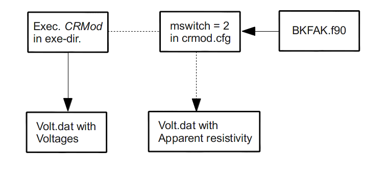
In order to use K-factors while modelling you can just do an integer switch at the last line of the crmod.cfg. For switching to the option wkfak insert a 2. After the Modelling with CRMod finished the third column of the crmod.cfg now represents the apparent resistivity \(\rho\).