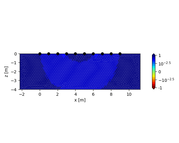
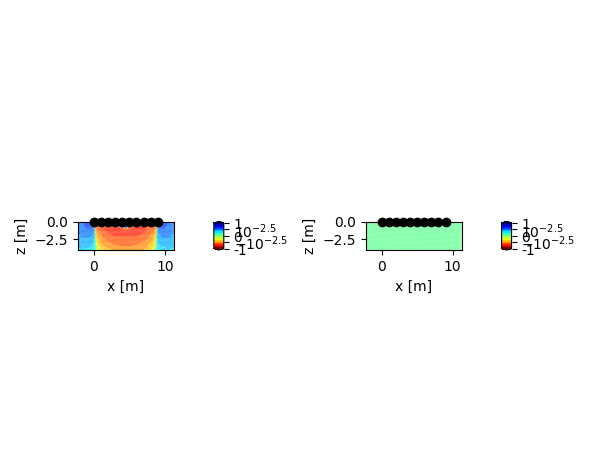
Plotting sensitivities

Sensitivity distributions can be easily plotted using the tdMan class:

imports

import numpy as np
import crtomo
# is only used for reda.CreateEnterDirectory
import reda

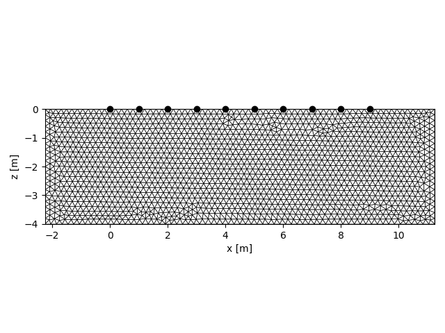
create and save a FEM-grid

grid = crtomo.crt_grid.create_surface_grid(
    nr_electrodes=8,
    spacing=1,
    # char_lengths=0.05,
    char_lengths=[0.05, 0.1, 0.1, 0.1],
    depth=8,
    left=5,
    right=5,
    internal_lines=[
        [4, -1, 6, -1],
        [4, -2, 6, -2],
        [4, -1, 4, -2],
        [6, -1, 6, -2],
        [0, -1, 3, -1],
        [0, -2, 3, -2],
        [0, -1, 0, -2],
        [3, -1, 3, -2],
    ],
)

fig, ax = grid.plot_grid()

with reda.CreateEnterDirectory('output_plot_00_sensitivity'):
    grid.save_elem_file('elem.dat')
    grid.save_elec_file('elec.dat')

This grid was sorted using CutMcK. The nodes were resorted!
Triangular grid found

create the measurement configuration

configs = np.array((
    (1, 2, 7, 6),
))

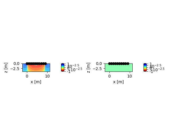
for different background, plot the sensitivities

for bg in (1, 10, 100, 1000):
    td = crtomo.tdMan(grid=grid)
    td.configs.add_to_configs(configs)
    pid_mag, pid_pha = td.add_homogeneous_model(bg, 0)

    from shapely.geometry import Polygon # noqa:402
    poly = Polygon([
        [4, -1],
        [6, -1],
        [6, -2],
        [4, -2],
    ])
    td.parman.modify_polygon(pid_mag, poly, 1)

    poly = Polygon([
        [0, -1],
        [3, -1],
        [3, -2],
        [0, -2],
    ])
    td.parman.modify_polygon(pid_pha, poly, -150)

    td.model(sensitivities=True, silent=True)

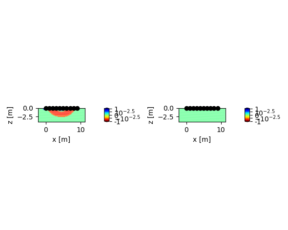
    # plot both mag and pha sensitivities
    fig, ax = td.plot_sensitivity(config_nr=0)
    with reda.CreateEnterDirectory('output_plot_00_sensitivity'):
        fig.savefig(
            'sensitivity_bg_{}.jpg'.format(bg),
            dpi=300,
            bbox_inches='tight'
        )

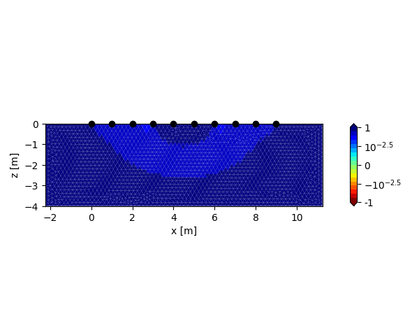
    # create another plot that only shows the magnitude sensitivity
    fig, ax = td.plot_sensitivity(config_nr=0, mag_only=True)
    with reda.CreateEnterDirectory('output_plot_00_sensitivity'):
        fig.savefig(
            'sensitivity_magonly_bg_{}.jpg'.format(bg),
            dpi=300,
            bbox_inches='tight'
        )

• 
• 
• 
• 
• 
• 
• 
• 

reading sensitivities
reading sensitivities
reading sensitivities
reading sensitivities