Note
Go to the end to download the full example code.
A single-frequency inversion (CR container)
Full processing of one frequency of one timestep of the data from Weigand and Kemna 2017 (Biogeosciences).
This example uses the CR container to load single-frequency data from a CRTomo-style volt.dat file.
imports
import os

import numpy as np

import crtomo
import reda
import reda.utils.geometric_factors as geom_facs
from reda.utils.fix_sign_with_K import fix_sign_with_K
import reda.importers.eit_fzj as eit_fzj
define an output directory for all files
output_directory = 'output_single_freq_inversion_CR'
cr = reda.CR()
cr.import_crtomo_data('data/volt.dat')
# this is a container measurement, we need to compute geometric factors using

# numerical modeling
# Note that this only works if CRMod is available
settings = {
    'rho': 100,
    'elem': 'data/elem.dat',
    'elec': 'data/elec.dat',
    'sink_node': '6467',
    '2D': True,
}
k = geom_facs.compute_K_numerical(cr.data, settings)
cr.data = geom_facs.apply_K(cr.data, k)
fix_sign_with_K(cr.data)
print(cr.data.iloc[0:5])
SETTINGS
{'rho': 100, 'elem': 'data/elem.dat', 'elec': 'data/elec.dat', 'sink_node': '6467', '2D': True}
2D modeling
   a   b   m   n  ...            k        rho_a   sigma_a             rho_a_complex
0  1   2  21  20  ...  9061.232484    46.166980  0.021661    40.270914+  22.575286j
1  1  27  30  28  ...     1.529047  1282.753055  0.000780  1282.753033-   0.235647j
2  1  27  31  29  ...     1.596560  1298.674366  0.000770  1298.674241-   0.569899j
3  1  27  32  28  ...     0.689674  1336.160025  0.000748  1336.159970-   0.383912j
4  1  27  32  30  ...     1.256348  1380.042077  0.000725  1380.041984-   0.505736j

[5 rows x 15 columns]
apply correction factors, as described in Weigand and Kemna, 2017 BG
corr_facs_nor = np.loadtxt('data/corr_fac_avg_nor.dat')
corr_facs_rec = np.loadtxt('data/corr_fac_avg_rec.dat')
corr_facs = np.vstack((corr_facs_nor, corr_facs_rec))
cr.data, cfacs = eit_fzj.apply_correction_factors(cr.data, corr_facs)
apply some filters import IPython IPython.embed()
cr.filter('r < 0')
cr.filter('rho_a < 15 or rho_a > 35')
cr.filter('rpha < - 40 or rpha > 3')
cr.filter('rphadiff < -5 or rphadiff > 5')
cr.filter('k > 400')
cr.filter('rho_a < 0')
cr.filter('a == 12 or b == 12 or m == 12 or n == 12')
cr.filter('a == 13 or b == 13 or m == 13 or n == 13')

# NOTE: this is also a single-frequency filtering,

cr.print_data_journal()
cr.print_log()
--- Data Journal Start ---
2026-05-07 11:49:19.168472
A filter was applied with query "r < 0". In total 15 records were removed
A filter was applied with query "rho_a < 15 or rho_a > 35". In total 394 records were removed
A filter was applied with query "rpha < - 40 or rpha > 3". In total 159 records were removed
A filter was applied with query "rphadiff < -5 or rphadiff > 5". In total 82 records were removed
A filter was applied with query "k > 400". In total 224 records were removed
A filter was applied with query "rho_a < 0". In total 0 records were removed
A filter was applied with query "a == 12 or b == 12 or m == 12 or n == 12". In total 36 records were removed
A filter was applied with query "a == 13 or b == 13 or m == 13 or n == 13". In total 33 records were removed
--- Data Journal End ---

2026-05-07 11:49:12,645 - reda.containers.BaseContainer - INFO - Data sized changed from 1925 to 1910
2026-05-07 11:49:13,814 - reda.containers.BaseContainer - INFO - Data sized changed from 1910 to 1516
2026-05-07 11:49:14,780 - reda.containers.BaseContainer - INFO - Data sized changed from 1516 to 1357
2026-05-07 11:49:15,675 - reda.containers.BaseContainer - INFO - Data sized changed from 1357 to 1275
2026-05-07 11:49:16,526 - reda.containers.BaseContainer - INFO - Data sized changed from 1275 to 1051
2026-05-07 11:49:17,206 - reda.containers.BaseContainer - INFO - Data sized changed from 1051 to 1051
2026-05-07 11:49:17,888 - reda.containers.BaseContainer - INFO - Data sized changed from 1051 to 1015
2026-05-07 11:49:18,541 - reda.containers.BaseContainer - INFO - Data sized changed from 1015 to 982
export to volt.dat file note that this is not required for the subsequent code
with reda.CreateEnterDirectory(output_directory):
    cr.export_crtomo('volt.dat', 'nor')
alternatively: directly create a tdman object that represents a single-frequency inversion with CRTomo
grid = crtomo.crt_grid('data/elem.dat', 'data/elec.dat')
tdman = cr.export_to_crtomo_td_manager(grid, norrec='nor')

# set inversion settings
tdman.crtomo_cfg['robust_inv'] = 'F'
tdman.crtomo_cfg['mag_abs'] = 0.012
tdman.crtomo_cfg['mag_rel'] = 0.5
tdman.crtomo_cfg['hom_bg'] = 'T'
tdman.crtomo_cfg['d2_5'] = 0
tdman.crtomo_cfg['fic_sink'] = 'T'
tdman.crtomo_cfg['fic_sink_node'] = 6467

# run the inversion, use the given output directory to store the CRTomo
# directory structure for later use
# only invert if the output directory does not exists
outdir = '{}/tomodir_inversion'.format(output_directory)
if not os.path.isdir(outdir):
    tdman.invert(
        catch_output=False,
        output_directory=outdir,
    )
else:
    tdman.read_inversion_results(outdir)
    print('Statistics of last iteration:')
    print(tdman.inv_stats.iloc[-1])
This grid was sorted using CutMcK. The nodes were resorted!
Rectangular grid found
Attempting inversion in directory: output_single_freq_inversion_CR/tomodir_inversion
Using binary: /usr/bin/CRTomo_dev
Calling CRTomo
Inversion attempt finished
Attempting to import the results
Reading inversion results
is robust False
Info: res_m.diag not found: output_single_freq_inversion_CR/tomodir_inversion/inv/res_m.diag
/home/runner/work/crtomo_tools/crtomo_tools/examples/02_simple_inversion
Info: ata.diag not found: output_single_freq_inversion_CR/tomodir_inversion/inv/ata.diag
/home/runner/work/crtomo_tools/crtomo_tools/examples/02_simple_inversion
Statistics of last iteration:
iteration              2
main_iteration         2
it_type            DC/IP
type                main
dataRMS              1.0
magRMS               1.0
phaRMS               0.0
lambda             476.2
roughness         0.4061
cgsteps             62.0
nrdata             477.0
steplength           0.0
stepsize           61.68
l1ratio              NaN
Name: 11, dtype: object
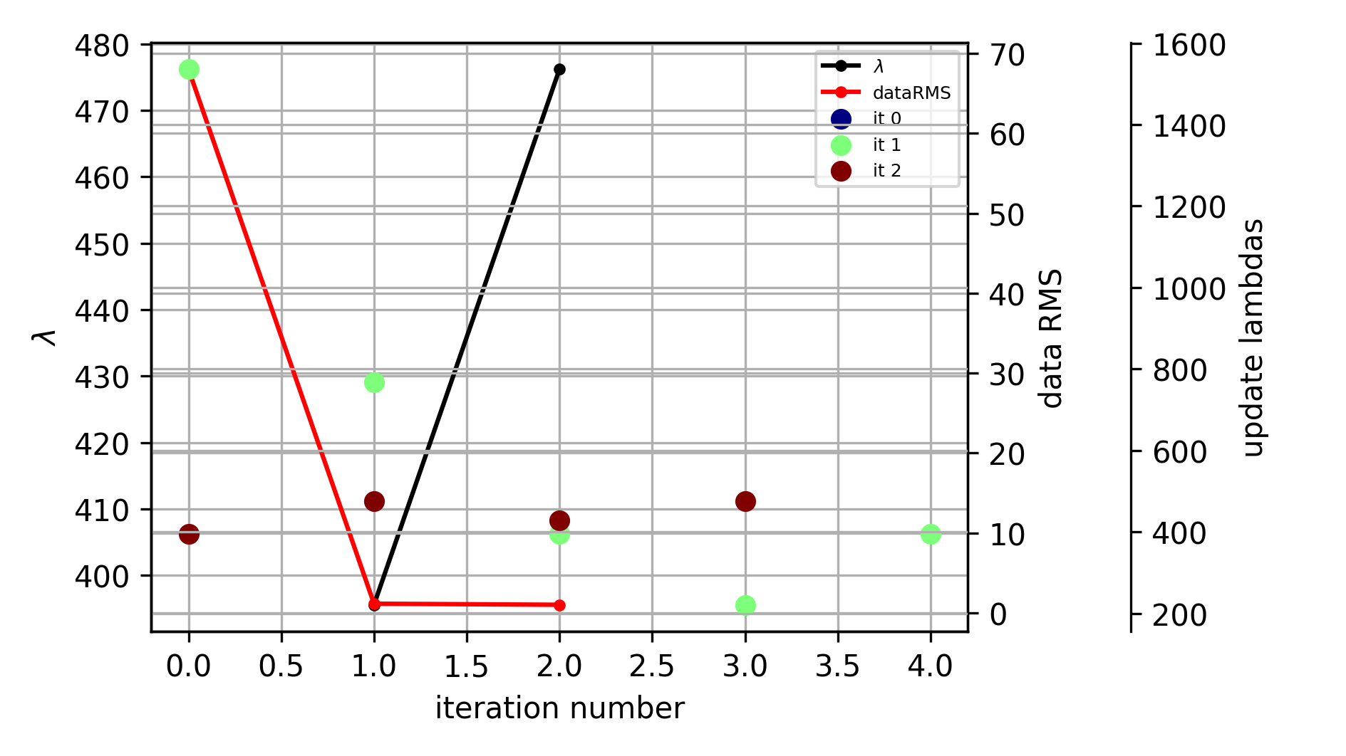
evolution of the inversion
fig = tdman.plot_inversion_evolution()
with reda.CreateEnterDirectory(output_directory):
    fig.savefig('inversion_evolution.png')

# the statistics are stored in a data frame
print(tdman.inv_stats)
print(tdman.inv_stats.columns)

#############################
0
Empty DataFrame
Columns: [iteration, main_iteration, it_type, type, dataRMS, magRMS, phaRMS, lambda, roughness, cgsteps, nrdata, steplength, stepsize, l1ratio]
Index: []
#############################
1
   iteration  main_iteration it_type  ... steplength  stepsize  l1ratio
1          1               1   DC/IP  ...        1.0    7440.0      NaN
2          2               1   DC/IP  ...        1.0    7370.0      NaN
3          3               1   DC/IP  ...        1.0    7290.0      NaN
4          4               1   DC/IP  ...        1.0    7200.0      NaN
5          5               1   DC/IP  ...        0.5    3650.0      NaN

[5 rows x 14 columns]
#############################
2
    iteration  main_iteration it_type  ... steplength  stepsize  l1ratio
7           0               2   DC/IP  ...        1.0      61.0      NaN
8           1               2   DC/IP  ...        1.0      61.7      NaN
9           2               2   DC/IP  ...        1.0      61.3      NaN
10          3               2   DC/IP  ...        0.5      30.8      NaN

[4 rows x 14 columns]
    iteration  main_iteration it_type  ... steplength  stepsize  l1ratio
0           0               0   DC/IP  ...        NaN       NaN      NaN
1           1               1   DC/IP  ...        1.0   7440.00      NaN
2           2               1   DC/IP  ...        1.0   7370.00      NaN
3           3               1   DC/IP  ...        1.0   7290.00      NaN
4           4               1   DC/IP  ...        1.0   7200.00      NaN
5           5               1   DC/IP  ...        0.5   3650.00      NaN
6           1               1   DC/IP  ...        3.0   7293.00      NaN
7           0               2   DC/IP  ...        1.0     61.00      NaN
8           1               2   DC/IP  ...        1.0     61.70      NaN
9           2               2   DC/IP  ...        1.0     61.30      NaN
10          3               2   DC/IP  ...        0.5     30.80      NaN
11          2               2   DC/IP  ...        0.0     61.68      NaN

[12 rows x 14 columns]
Index(['iteration', 'main_iteration', 'it_type', 'type', 'dataRMS', 'magRMS',
       'phaRMS', 'lambda', 'roughness', 'cgsteps', 'nrdata', 'steplength',
       'stepsize', 'l1ratio'],
      dtype='object')
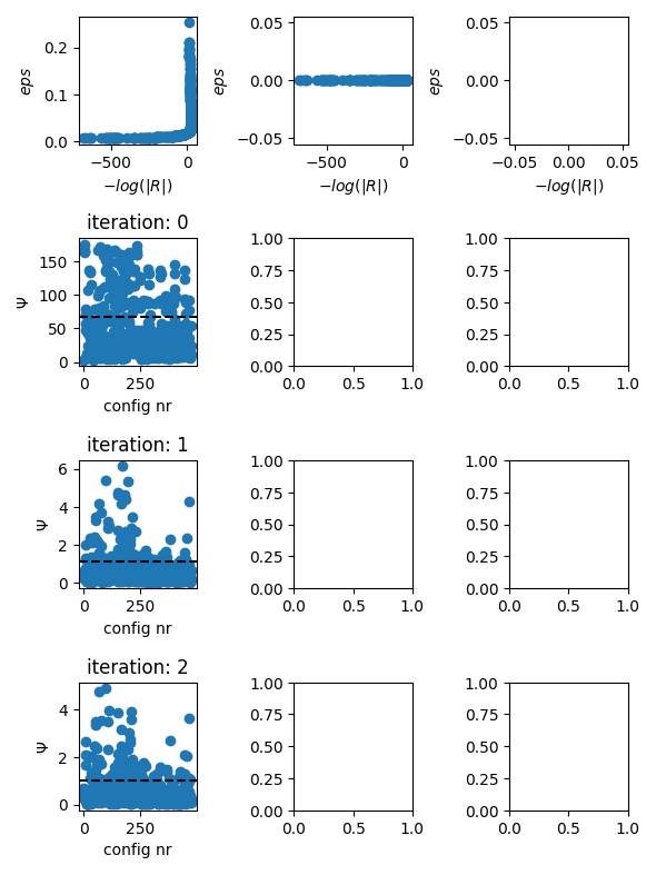
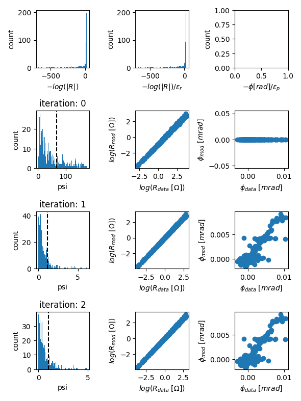
evolution of data misfits
fig = tdman.plot_eps_data()
fig = tdman.plot_eps_data_hist()

# eps data is found here:
tdman.eps_data
r = tdman.plot.plot_elements_to_ax(
    tdman.a['inversion']['rmag'][-1],
    plot_colorbar=True,
    cmap_name='jet_r',
)
with reda.CreateEnterDirectory(output_directory):
    r[0].savefig('rmag.png', bbox_inches='tight')

r = tdman.plot.plot_elements_to_ax(
    tdman.a['inversion']['rpha'][-1],
    plot_colorbar=True,
    cmap_name='jet_r',
)
with reda.CreateEnterDirectory(output_directory):
    r[0].savefig('rpha_last_it.png', bbox_inches='tight')
Total running time of the script: (2 minutes 24.310 seconds)


