Plot forward models

Test plotting forward models for different mesh boundaries.

imports

import numpy as np
import crtomo

set up plotting facilities - this will often generate better fitting plots

import crtomo.mpl
crtomo.mpl.setup()

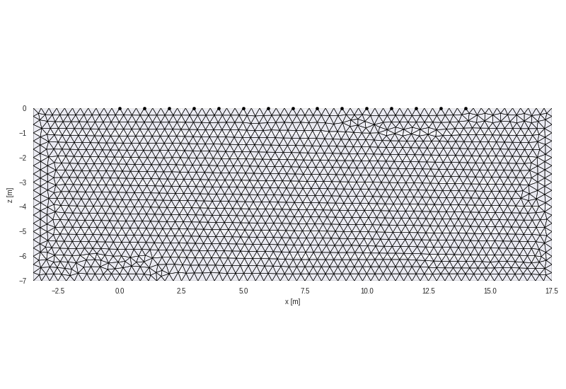
a surface grid

grid = crtomo.crt_grid.create_surface_grid(nr_electrodes=15, spacing=1)
grid.plot_grid()
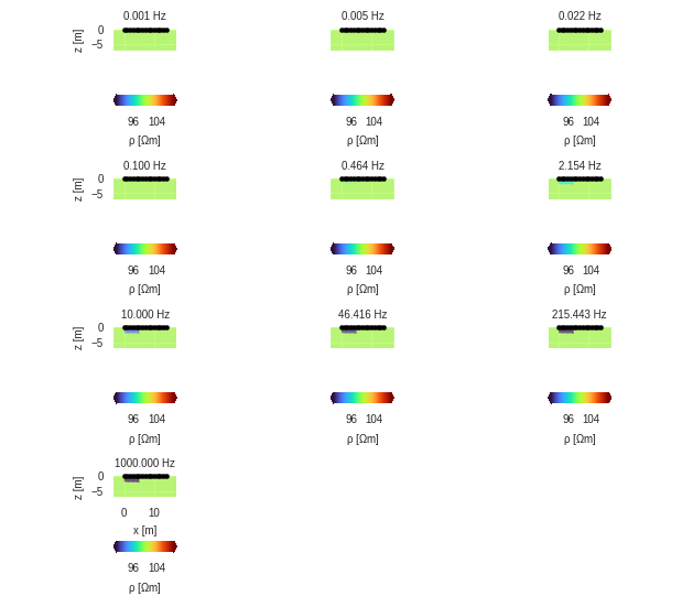
frequencies = np.logspace(-3, 3, 10)
eitman = crtomo.eitMan(frequencies=frequencies, grid=grid)
eitman.add_homogeneous_model(magnitude=100, phase=0)
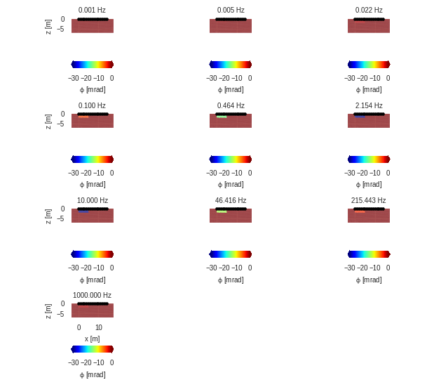
eitman.set_area_to_single_colecole(
    0, 5, -2, 0,
    [100, 0.1, 0.04, 0.8]
)
r = eitman.plot_forward_models(maglim=[90, 110], phalim=[-30, 0])

# save to files
r['rpha']['fig'].savefig('fwd_model_par_rpha.png', dpi=300)

• 
• 
• 

This grid was sorted using CutMcK. The nodes were resorted!
Triangular grid found

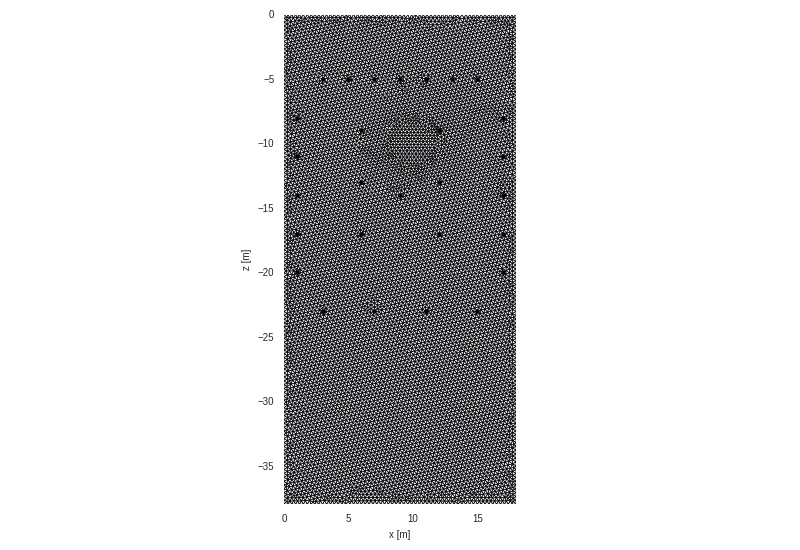
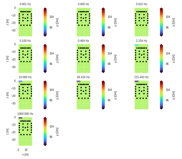
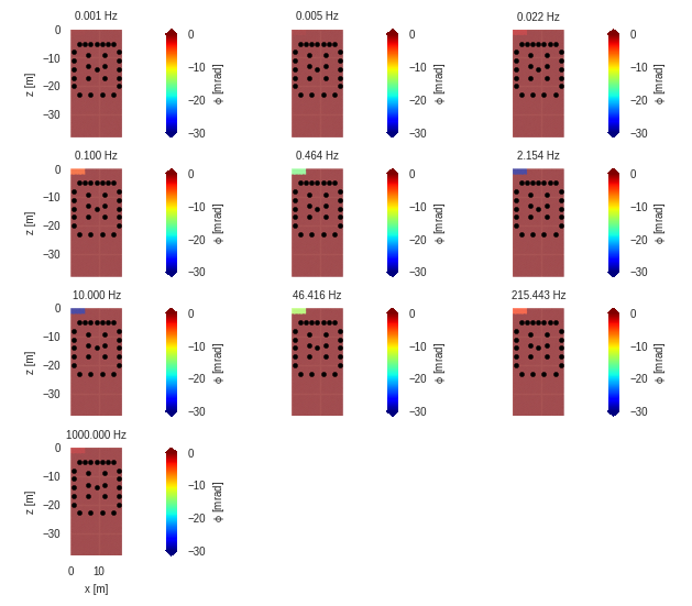
a rhizotron

grid = crtomo.crt_grid('grid_rhizotron/elem.dat', 'grid_rhizotron/elec.dat')

grid.plot_grid()
frequencies = np.logspace(-3, 3, 10)
eitman = crtomo.eitMan(frequencies=frequencies, grid=grid)
eitman.add_homogeneous_model(magnitude=100, phase=0)
eitman.set_area_to_single_colecole(
    0, 5, -2, 0,
    [100, 0.1, 0.04, 0.8]
)
r = eitman.plot_forward_models(maglim=[90, 110], phalim=[-30, 0])

# save to files
# r['rpha']['fig'].savefig('fwd_model_par_rpha.png', dpi=300)
# sphinx_gallery_thumbnail_number = -1

• 
• 
• 

This grid was sorted using CutMcK. The nodes were resorted!
Triangular grid found