Note
Go to the end to download the full example code.
A single-frequency inversion (sEIT container)
Full processing of one frequency of one timestep of the data from Weigand and Kemna 2017 (Biogeosciences).
This example uses the sEIT container to load multi-frequency data from the original measurement data.
imports
import os

import numpy as np

import reda
import reda.utils.geometric_factors as geom_facs
from reda.utils.fix_sign_with_K import fix_sign_with_K
import reda.importers.eit_fzj as eit_fzj
define an output directory for all files
output_directory = 'output_single_freq_inversion_sEIT'
import the sEIT data set
seit = reda.sEIT()
seit.import_eit_fzj(
    'data/bnk_raps_20130408_1715_03_einzel.mat',
    'data/configs.dat'
)
Constructing four-point measurements
Summary:
                  a             b  ...     frequency          rpha
count  67375.000000  67375.000000  ...  67375.000000  67375.000000
mean      17.907532     20.831169  ...   2577.580109    473.723981
std       10.333167     10.677015  ...   8258.716055   2729.735973
min        1.000000      2.000000  ...      0.462963  -3141.592649
25%       10.000000     12.000000  ...     29.411765  -3131.399200
50%       17.000000     22.000000  ...    122.222220      5.510219
75%       27.000000     30.000000  ...    700.000000   3139.297772
max       37.000000     38.000000  ...  45000.000000   3141.592652

[8 rows x 7 columns]
with reda.CreateEnterDirectory(output_directory):
    # export the data into CRTomo-style data files. Each frequency gets its own
    # file
    seit.export_to_crtomo_multi_frequency('result_raw_data')

    # just for demonstration purposes, data could be imported from this
    # directory:
    # create a new sEIT container
    seit_temp = reda.sEIT()
    seit_temp.import_crtomo('result_raw_data')
    # delete it to prevent any confusions
    del(seit_temp)
Summary:
                  a             b  ...     frequency          rpha
count  67375.000000  67375.000000  ...  67375.000000  67375.000000
mean      17.907532     20.831169  ...   2577.580109    473.723981
std       10.333167     10.677015  ...   8258.716055   2729.735973
min        1.000000      2.000000  ...      0.462963  -3141.592649
25%       10.000000     12.000000  ...     29.411765  -3131.399201
50%       17.000000     22.000000  ...    122.222220      5.510219
75%       27.000000     30.000000  ...    700.000000   3139.297772
max       37.000000     38.000000  ...  45000.000000   3141.592652

[8 rows x 7 columns]
this is a container measurement, we need to compute geometric factors using numerical modeling Note that this only work if CRMod is available
SETTINGS
{'rho': 100, 'elem': 'data/elem.dat', 'elec': 'data/elec.dat', 'sink_node': '6467', '2D': True}
2D modeling
apply correction factors, as described in Weigand and Kemna, 2017 BG
corr_facs_nor = np.loadtxt('data/corr_fac_avg_nor.dat')
corr_facs_rec = np.loadtxt('data/corr_fac_avg_rec.dat')
corr_facs = np.vstack((corr_facs_nor, corr_facs_rec))
seit.data, cfacs = eit_fzj.apply_correction_factors(seit.data, corr_facs)
apply some filters import IPython IPython.embed()
seit.filter('r < 0')
seit.filter('rho_a < 15 or rho_a > 35')
seit.filter('rpha < - 40 or rpha > 3')
seit.filter('rphadiff < -5 or rphadiff > 5')
seit.filter('k > 400')
seit.filter('rho_a < 0')
seit.filter('a == 12 or b == 12 or m == 12 or n == 12')
seit.filter('a == 13 or b == 13 or m == 13 or n == 13')

# seit.filter_incomplete_spectra(flimit=300, percAccept=85)
seit.print_data_journal()
seit.print_log()
--- Data Journal Start ---
2026-06-25 12:20:57.869866
A filter was applied with query "r < 0". In total 543 records were removed
A filter was applied with query "rho_a < 15 or rho_a > 35". In total 13919 records were removed
A filter was applied with query "rpha < - 40 or rpha > 3". In total 10016 records were removed
A filter was applied with query "rphadiff < -5 or rphadiff > 5". In total 14451 records were removed
A filter was applied with query "k > 400". In total 3619 records were removed
A filter was applied with query "rho_a < 0". In total 0 records were removed
A filter was applied with query "a == 12 or b == 12 or m == 12 or n == 12". In total 1003 records were removed
A filter was applied with query "a == 13 or b == 13 or m == 13 or n == 13". In total 934 records were removed
--- Data Journal End ---

2026-06-25 12:20:57,825 - reda.main.logger - INFO - Data sized changed from 67375 to 66832
2026-06-25 12:20:57,833 - reda.main.logger - INFO - Data sized changed from 66832 to 52913
2026-06-25 12:20:57,840 - reda.main.logger - INFO - Data sized changed from 52913 to 42897
2026-06-25 12:20:57,847 - reda.main.logger - INFO - Data sized changed from 42897 to 28446
2026-06-25 12:20:57,852 - reda.main.logger - INFO - Data sized changed from 28446 to 24827
2026-06-25 12:20:57,857 - reda.main.logger - INFO - Data sized changed from 24827 to 24827
2026-06-25 12:20:57,863 - reda.main.logger - INFO - Data sized changed from 24827 to 23824
2026-06-25 12:20:57,869 - reda.main.logger - INFO - Data sized changed from 23824 to 22890
export normal data to volt.dat file note that this is not required for the subsequent code and could be completely removed !!!
with reda.CreateEnterDirectory(output_directory):
    seit.export_to_crtomo_one_frequency('volt.dat', 70.0, 'nor')
alternatively: directly create a tdman object that represents a single-frequency inversion with CRTomo
import crtomo
grid = crtomo.crt_grid('data/elem.dat', 'data/elec.dat')
tdman = seit.export_to_crtomo_td_manager(grid, frequency=70.0, norrec='nor')

# set inversion settings
tdman.crtomo_cfg['robust_inv'] = 'F'
tdman.crtomo_cfg['mag_abs'] = 0.012
tdman.crtomo_cfg['mag_rel'] = 0.5
tdman.crtomo_cfg['hom_bg'] = 'T'
tdman.crtomo_cfg['d2_5'] = 0
tdman.crtomo_cfg['fic_sink'] = 'T'
tdman.crtomo_cfg['fic_sink_node'] = 6467

# run the inversion, use the given output directory to store the CRTomo
# directory structure for later use
# only invert if the output directory does not exists
outdir = '{}/tomodir_inversion'.format(output_directory)
if not os.path.isdir(outdir):
    tdman.invert(
        catch_output=False,
        output_directory=outdir,
    )
else:
    tdman.read_inversion_results(outdir)
    print('Statistics of last iteration:')
    print(tdman.inv_stats.iloc[-1])
This grid was sorted using CutMcK. The nodes were resorted!
Rectangular grid found
Attempting inversion in directory: output_single_freq_inversion_sEIT/tomodir_inversion
Using binary: /home/runner/.virtualenvs/crtomo/bin/CRTomo
Calling CRTomo
b' ######### CRTomo ############\nLicence:\nCopyright \xc2\xa9 1990-2020 Andreas Kemna <kemna@geo.uni-bonn.de>\nCopyright \xc2\xa9 2008-2020 CRTomo development team (see AUTHORS file)\nPermission is hereby granted, free of charge, to any person obtaining a copy of\nthis software and associated documentation files (the \xe2\x80\x9cSoftware\xe2\x80\x9d), to deal in\nthe Software without restriction, including without limitation the rights to\nuse, copy, modify, merge, publish, distribute, sublicense, and/or sell copies\nof the Software, and to permit persons to whom the Software is furnished to do\nso, subject to the following conditions:\n\nThe above copyright notice and this permission notice shall be included in all\ncopies or substantial portions of the Software.\n\nTHE SOFTWARE IS PROVIDED \xe2\x80\x9cAS IS\xe2\x80\x9d, WITHOUT WARRANTY OF ANY KIND, EXPRESS OR\nIMPLIED, INCLUDING BUT NOT LIMITED TO THE WARRANTIES OF MERCHANTABILITY,\nFITNESS FOR A PARTICULAR PURPOSE AND NONINFRINGEMENT. IN NO EVENT SHALL THE\nAUTHORS OR COPYRIGHT HOLDERS BE LIABLE FOR ANY CLAIM, DAMAGES OR OTHER\nLIABILITY, WHETHER IN AN ACTION OF CONTRACT, TORT OR OTHERWISE, ARISING FROM,\nOUT OF OR IN CONNECTION WITH THE SOFTWARE OR THE USE OR OTHER DEALINGS IN THE\nSOFTWARE.\n \n \n Process_ID :: 5858\n OpenMP max threads: 2\n Version control of binary:\n Git-Branch meson_f2py\n Commit-ID dbe2f7d238dfd4d5c3eb291966f52caf629bd2c9\n Created Sun-May-11-20:40:39-2025\n Compiler \n OS GNU/Linux\n\nOS identification: Linux-OS\n writing inversion results into ../inv\n ## using complex error ellipses ##\n++ check 1\r++ check 2 done!\n\nFictious sink @ node 6467 31.000 -53.000\n\n + Taking error model\n\n+++ Found no presettings for lambda_0 (default)\n\n Saving lamba presettings -> crt.lamnull\n\n++ (CRI) Setting complex error ellipse\n\n\n\n2D without Dirichlet nodes setting k=1e-6\n OpenMP threads: 2( 2)\n\r \r Iteration 0, 0 : Calculating Potentials++ Starting Fit 73.37 \n\n\n\rWRITING STARTING MODEL\n\n\r \r Iteration 1, 0 : Calculating Sensitivities\nRegularization:: Triangular smooth\n C_m^ calculation time\n C_m^ calculation time 0d/ 0h/ 0m/ 0s/ 1ms\n\r Iteration 1, 1 : Calculating 1st regularization parameter \r found lam_0 1358. \nlam_0:: 0.14E+04\r \r Iteration 1, 1 : Updating\r \r Iteration 1, 1 : Calculating Potentials -- Update Fit 1.128 \r \r Iteration 1, 2 : Updating\r \r Iteration 1, 2 : Calculating Potentials -- Update Fit 1.135 \r \r Iteration 1, 3 : Updating\r \r Iteration 1, 3 : Calculating Potentials -- Update Fit 36.71 \r \r Iteration 1, 3 : Updating\r \r Iteration 1, 3 : Calculating Potentials ++ Actual Fit 1.128 \n\n+++ Convergence check (CHI (old/new)) -6403. %\n\n\r \r Iteration 2, 0 : Calculating Sensitivities\r \r Iteration 2, 0 : Updating\r \r Iteration 2, 0 : Calculating Potentials -- Update Fit 1.148 \r \r Iteration 2, 1 : Updating\r \r Iteration 2, 1 : Calculating Potentials -- Update Fit 1.020 \r \r Iteration 2, 2 : Updating\r \r Iteration 2, 2 : Calculating Potentials -- Update Fit 0.9888 \r \r Iteration 2, 3 : Updating\r \r Iteration 2, 3 : Calculating Potentials -- Update Fit 1.014 \r \r Iteration 2, 4 : Updating\r \r Iteration 2, 4 : Calculating Potentials -- Update Fit 1.048 \r \r Iteration 2, 4 : Updating\r \r Iteration 2, 4 : Calculating Potentials ++ Actual Fit 0.9981 \n\n+++ Convergence check (CHI (old/new)) -13.04 %\n\n\r \r Iteration 3, 0 : Calculating Sensitivities\r \r Iteration 3, 0 : Updating\r \r Iteration 3, 0 : Calculating Potentials -- Update Fit 0.9874 \r \r Iteration 3, 1 : Updating\r \r Iteration 3, 1 : Calculating Potentials -- Update Fit 1.013 \r \r Iteration 3, 2 : Updating\r \r Iteration 3, 2 : Calculating Potentials -- Update Fit 0.9926 \r \r Iteration 3, 2 : Updating\r \r Iteration 3, 2 : Calculating Potentials ++ Actual Fit 0.9981 \n\n+++ Convergence check (CHI (old/new)) -0.1116E-02 %\n\n\rMODEL ESTIMATE AFTER 3 ITERATIONS \n Iteration terminated: Min. rel. CHI decrease.\n CPU time:\n CPU time: 0d/ 0h/ 1m/ 51s/ 934ms\n ***finished***\n'
Inversion attempt finished
Attempting to import the results
Reading inversion results
is robust False
Info: res_m.diag not found: output_single_freq_inversion_sEIT/tomodir_inversion/inv/res_m.diag
/home/runner/work/crtomo_tools/crtomo_tools/examples/02_simple_inversion
Info: ata.diag not found: output_single_freq_inversion_sEIT/tomodir_inversion/inv/ata.diag
/home/runner/work/crtomo_tools/crtomo_tools/examples/02_simple_inversion
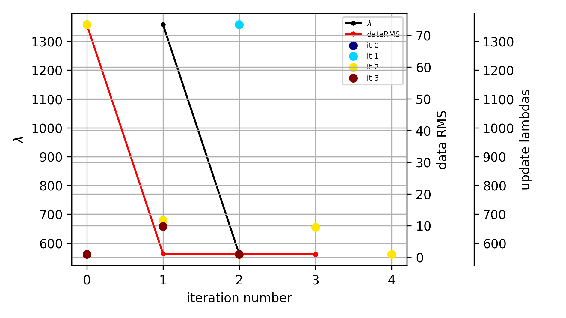
Statistics of last iteration:
iteration 3
main_iteration 3
it_type DC/IP
type main
dataRMS 0.9981
magRMS 0.9
phaRMS 9.0
lambda 561.3
roughness 0.3254
cgsteps 70.0
nrdata 354.0
steplength 9.0
stepsize 0.000066
l1ratio NaN
Name: 14, dtype: object
evolution of the inversion
fig = tdman.plot_inversion_evolution()
with reda.CreateEnterDirectory(output_directory):
    fig.savefig('inversion_evolution.png')

# the statistics are stored in a data frame
print(tdman.inv_stats)
print(tdman.inv_stats.columns)
#############################
0
Empty DataFrame
Columns: [iteration, main_iteration, it_type, type, dataRMS, magRMS, phaRMS, lambda, roughness, cgsteps, nrdata, steplength, stepsize, l1ratio]
Index: []
#############################
1
   iteration  main_iteration it_type  ... steplength  stepsize  l1ratio
1          1               1   DC/IP  ...        1.0    7420.0      NaN
2          2               1   DC/IP  ...        1.0    7340.0      NaN
3          3               1   DC/IP  ...        0.5    3710.0      NaN

[3 rows x 14 columns]
#############################
2
   iteration  main_iteration it_type  ... steplength  stepsize  l1ratio
5          0               2   DC/IP  ...        1.0     11.00      NaN
6          1               2   DC/IP  ...        1.0      9.52      NaN
7          2               2   DC/IP  ...        1.0      9.19      NaN
8          3               2   DC/IP  ...        1.0      9.46      NaN
9          4               2   DC/IP  ...        0.5      4.59      NaN

[5 rows x 14 columns]
#############################
3
    iteration  main_iteration it_type  ... steplength  stepsize  l1ratio
11          0               3   DC/IP  ...        1.0    0.0656      NaN
12          1               3   DC/IP  ...        1.0    0.1060      NaN
13          2               3   DC/IP  ...        0.5    0.0328      NaN

[3 rows x 14 columns]
    iteration  main_iteration it_type  ... steplength     stepsize  l1ratio
0           0               0   DC/IP  ...        NaN          NaN      NaN
1           1               1   DC/IP  ...        1.0  7420.000000      NaN
2           2               1   DC/IP  ...        1.0  7340.000000      NaN
3           3               1   DC/IP  ...        0.5  3710.000000      NaN
4           1               1   DC/IP  ...        8.0  7421.000000      NaN
5           0               2   DC/IP  ...        1.0    11.000000      NaN
6           1               2   DC/IP  ...        1.0     9.520000      NaN
7           2               2   DC/IP  ...        1.0     9.190000      NaN
8           3               2   DC/IP  ...        1.0     9.460000      NaN
9           4               2   DC/IP  ...        0.5     4.590000      NaN
10          2               2   DC/IP  ...        9.0     8.314000      NaN
11          0               3   DC/IP  ...        1.0     0.065600      NaN
12          1               3   DC/IP  ...        1.0     0.106000      NaN
13          2               3   DC/IP  ...        0.5     0.032800      NaN
14          3               3   DC/IP  ...        9.0     0.000066      NaN

[15 rows x 14 columns]
Index(['iteration', 'main_iteration', 'it_type', 'type', 'dataRMS', 'magRMS',
       'phaRMS', 'lambda', 'roughness', 'cgsteps', 'nrdata', 'steplength',
       'stepsize', 'l1ratio'],
      dtype='object')
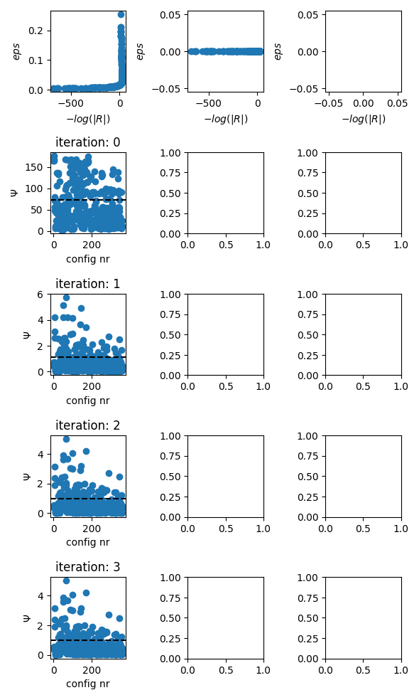
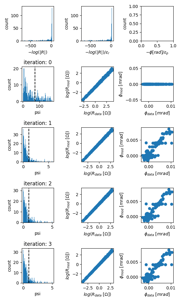
evolution of data misfits
fig = tdman.plot_eps_data()
fig = tdman.plot_eps_data_hist()

# eps data is found here:
tdman.eps_data
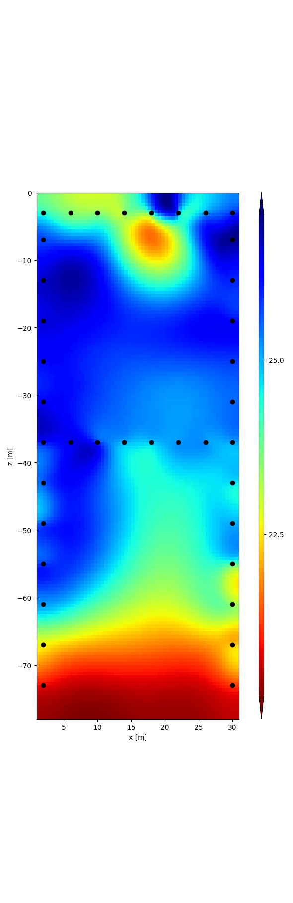
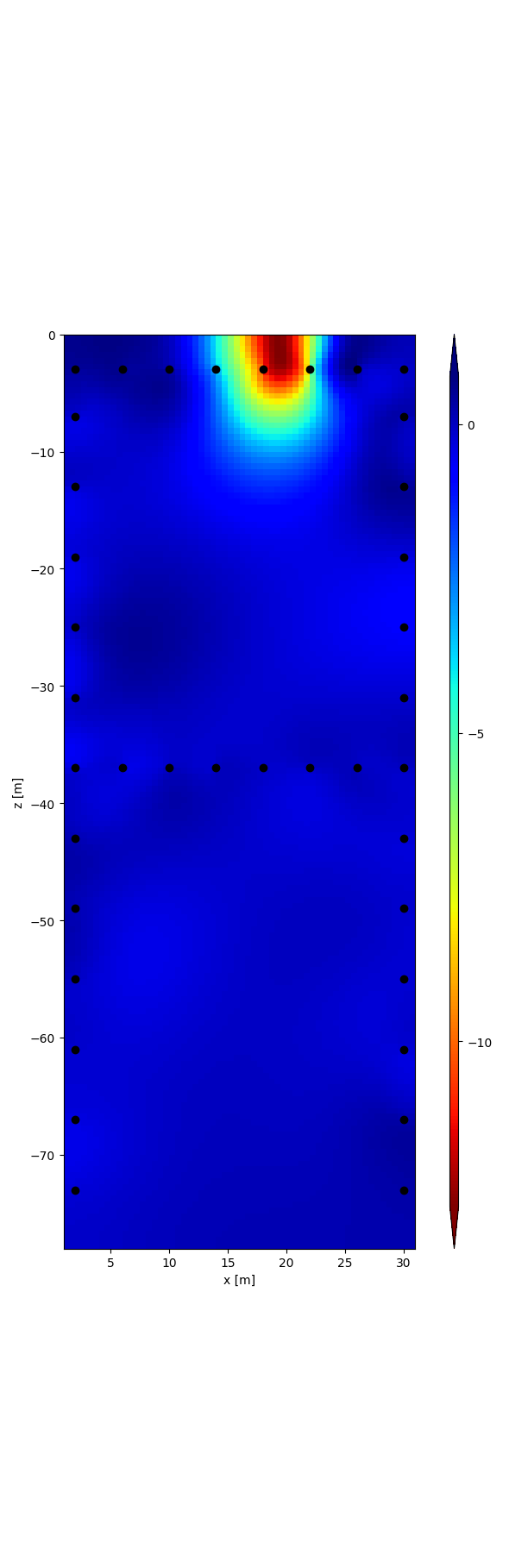
r = tdman.plot.plot_elements_to_ax(
    tdman.a['inversion']['rmag'][-1],
    plot_colorbar=True,
    cmap_name='jet_r',
)
with reda.CreateEnterDirectory(output_directory):
    r[0].savefig('rmag.png', bbox_inches='tight')

r = tdman.plot.plot_elements_to_ax(
    tdman.a['inversion']['rpha'][-1],
    plot_colorbar=True,
    cmap_name='jet_r',
)
with reda.CreateEnterDirectory(output_directory):
    r[0].savefig('rpha_last_it.png', bbox_inches='tight')
Total running time of the script: (2 minutes 32.908 seconds)