Modify a subsurface model

A subsurface model is basically an array of the same length as the number of model cells in the finite-element mesh. We refer to such an array as a parameter set (or parset), and the numeric (integer) id that refers to such as parset in the parameter manager as a pid. For DC forward modeling you only need one resistivity model (with M resistivity values for the M model cells), while for complex resistivity modeling you need a resistivity and a phase array.

Parameter sets are usually manager using the parameter manger class crtomo.parManager.ParMan, which also has an alias to crtomo.ParMan.

If you are using a single-frequency tomodir object tdm (crtomo.tdMan), one parameter manager is already initialized as tdm.parman.

There are various ways to modify such an array

• modify by index: crtomo.parManager.ParMan.modify_pixels()

• modify rectangular area: crtomo.parManager.ParMan.modify_area()

• modify by polygon crtomo.parManager.ParMan.modify_polygon()

• add Gaussian anomalies. See this example here: Generate Gaussian Models

• there is also the possibility to generate meshes that incorporate certain subsurface structures. See this example: Using Inkscape to define internal structure

import crtomo
import matplotlib.pylab as plt

load a mesh file that we want to create a model for

grid = crtomo.crt_grid('grid_surface/elem.dat', 'grid_surface/elec.dat')
# create a parameter manager
parman = crtomo.ParMan(grid)

This grid was sorted using CutMcK. The nodes were resorted!
Triangular grid found

we need a plot manager to plot our mesh/model parameters notice that we link the parameter manager to the plot manager

plotman = crtomo.pltMan(grid=grid, pm=parman)

create an empty parameter set

pid_mag = parman.add_empty_dataset(value=100)

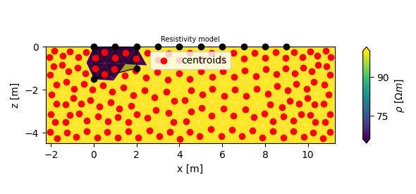
Modify by polygon

Probably the most versatile method to modify a subsurface model is by selecting cells using a polygon outline. The relevant function for this is crtomo.parManager.ParMan.modify_polygon() Note that only cells are selected whose center ob mass is located within the polygon!

It is advisable to create meshes that include the relevant polygon lines in the mesh. Note that those meshes should only be used for forward modeling, not for inverse modeling. For advanced grid creating, please refer to Irregular grids, especially the inclusion of extra lines: extra_lines.dat (optional).

from shapely.geometry import Polygon # noqa:402
poly = Polygon([
    [0, 0],
    [2, 0],
    [2, -1],
    [0, -1.5],
])
parman.modify_polygon(pid_mag, poly, 66)

fig, ax = plt.subplots(figsize=(15 / 2.54, 7 / 2.54))
plotman.plot_elements_to_ax(
    pid_mag,
    ax=ax,
    plot_colorbar=True,
    cblabel=r'$\rho~[\Omega m]$',
    title='Resistivity model'
)
# lets draw the original polygon
from shapely.plotting import plot_polygon # noqa: 402
plot_polygon(poly, ax=ax, color='k')

# lets plot the center of masses
ax.scatter(
    grid.get_element_centroids()[:, 0],
    grid.get_element_centroids()[:, 1],
    color='r',
    label='centroids',
)
ax.legend()
fig.tight_layout()
fig.savefig('out_03_model.jpg', dpi=300)