Plot a potential distribution

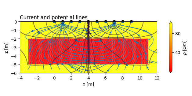
CRMod can return the potential distribution associated with the current electrode locations of each registered quadrupole. We can retrieve those potentials using the tdMan object and plot them. The current distribution can then be computed TODO

Imports

import numpy as np
import pylab as plt

import crtomo

create a tomodir object from an existing FE mesh

grid = crtomo.crt_grid(
    'grid_surface/g2_large_boundary/elem.dat',
    'grid_surface/g2_large_boundary/elec.dat'
)
td = crtomo.tdMan(grid=grid)

This grid was sorted using CutMcK. The nodes were resorted!
Triangular grid found

define configurations

td.configs.add_to_configs(
    np.array((
        (2, 8, 5, 7),
        (1, 3, 10, 7),
    ))
)

add a forward model with a conductive region

pid_mag, pid_pha = td.add_homogeneous_model(100, -50)
td.parman.modify_area(
    pid_mag,
    -3, 11,
    -5, -2,
    1,
)

compute FEM solution using CRMod

td.model(potentials=True)

attempting modeling
b' ######### CMod ############\nLicence:\nCopyright \xc2\xa9 1990-2020 Andreas Kemna <kemna@geo.uni-bonn.de>\nCopyright \xc2\xa9 2008-2020 CRTomo development team (see AUTHORS file)\nPermission is hereby granted, free of charge, to any person obtaining a copy of\nthis software and associated documentation files (the \xe2\x80\x9cSoftware\xe2\x80\x9d), to deal in\nthe Software without restriction, including without limitation the rights to\nuse, copy, modify, merge, publish, distribute, sublicense, and/or sell copies\nof the Software, and to permit persons to whom the Software is furnished to do\nso, subject to the following conditions:\n\nThe above copyright notice and this permission notice shall be included in all\ncopies or substantial portions of the Software.\n\nTHE SOFTWARE IS PROVIDED \xe2\x80\x9cAS IS\xe2\x80\x9d, WITHOUT WARRANTY OF ANY KIND, EXPRESS OR\nIMPLIED, INCLUDING BUT NOT LIMITED TO THE WARRANTIES OF MERCHANTABILITY,\nFITNESS FOR A PARTICULAR PURPOSE AND NONINFRINGEMENT. IN NO EVENT SHALL THE\nAUTHORS OR COPYRIGHT HOLDERS BE LIABLE FOR ANY CLAIM, DAMAGES OR OTHER\nLIABILITY, WHETHER IN AN ACTION OF CONTRACT, TORT OR OTHERWISE, ARISING FROM,\nOUT OF OR IN CONNECTION WITH THE SOFTWARE OR THE USE OR OTHER DEALINGS IN THE\nSOFTWARE.\n \n \n CRMod Process_ID ::        4827\n OpenMP max threads:   4\n Git-Branch  master\n Commit-ID   cb89ccd2c4341b9b08bbe7bb08f5aea0d60916ee\n Created     Mon-Mar-25-14:34:56-2024\n Compiler    \n OS          GNU/Linux\n\n Reading Input-Files\n++ check 1\r++ check 2 done!\n\rGetting voltage      1\rGetting voltage      2 No electrode cap file\n \n Rescheduling..\n less nodes than wavenumbers\n OpenMP threads:   3(  4)\n\n\r Calculating Potentials : Wavenumber          2                                                   \r Calculating Potentials : Wavenumber          2                                                   \r Calculating Potentials : Wavenumber          3                                                   \r Calculating Potentials : Wavenumber          4                                                   \r Calculating Potentials : Wavenumber          5                                                   \r Calculating Potentials : Wavenumber          6                                                   \r Calculating Potentials : Wavenumber          7                                                   \r Calculating Potentials : Wavenumber          8                                                   \r Calculating Potentials : Wavenumber          9                                                    done, now processing\n\rPotential :     50.00 %\rPotential :    100.00 % solution time  0d/  0h/  0m/  0s/ 938ms\n\n Modelling completedSTOP 0\n'
reading voltages
reading potentials

retrieve the potential distribution of the first quadrupole the potential distribution is returned as real and imaginary part

pot_re, pot_im = td.get_potential(0)
pot_mag = np.sqrt(
    pot_re ** 2 + pot_im ** 2
)

# add node data to the parameter manager
# for visualization purposes, we also store a transformed potential
# distribution
nid = td.nodeman.add_data(pot_re)
nid_asinh = td.nodeman.add_data(
    crtomo.plotManager.converter_asinh(pot_re)
)

# Create a nice plot
fig, ax = plt.subplots(1, 1, figsize=(16 / 2.54, 8 / 2.54), sharex=True)
ax.set_title('Current and potential lines', loc='left')

# plot the resistivity distribution of the forward model
td.plot.plot_elements_to_ax(
    pid_mag,
    ax,
    plot_colorbar=True,
    cmap='jet',
    cmap_name='autumn',
    cblabel=r'$\rho~[\Omega m]$',
)

# plot current lines
td.plot.plot_nodes_current_streamlines_to_ax(
    ax,
    # nid_asinh,
    nid,
    pid_mag,
    density=0.6,
)

# plot potential lines (contour lines)
# Note that we use the asinh-transformed potentials here. This ensures nicer
# looking potential lines
td.plot.plot_nodes_contour_to_ax(
    ax,
    nid_asinh,
    # nid,
    plot_colorbar=False,
    fill_contours=False,
    cblevels=21,
    alpha=0.6,
)

ax.set_aspect('equal')

fig.tight_layout()
fig.savefig('out_02_potential_distribution.jpg', dpi=300)