Note
Go to the end to download the full example code.
Forward Modeling with CRMod
Imports
import crtomo
create a tomodir object from an existing FE mesh
mesh = crtomo.crt_grid(
    'grid_surface/g2_large_boundary/elem.dat',
    'grid_surface/g2_large_boundary/elec.dat'
)
This grid was sorted using CutMcK. The nodes were resorted!
Triangular grid found
create a tomodir-manager object this object will hold everything required for modeling and inversion runs
tdm = crtomo.tdMan(grid=mesh)
generate measurement configurations
tdm.configs.gen_dipole_dipole(skipc=0)
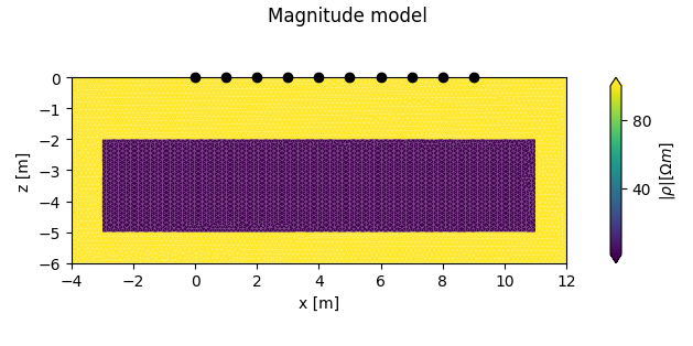
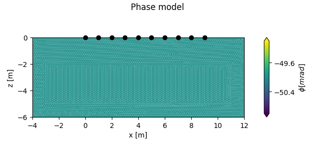
add a forward model with a conductive region
plot the forward models
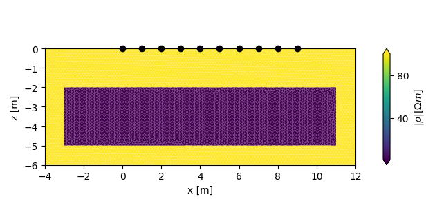
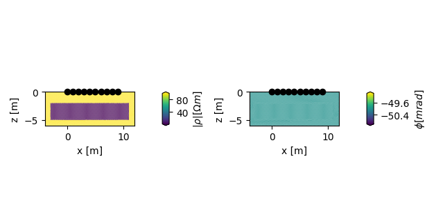
Two lists are returned, each containing either two figures, or two axes
Compute FEM solution using CRMod:
tdm.model(silent=True)
measurements can now be retrieved First column: resistances, second column: phase values [mrad]
measurements = tdm.measurements()
print(measurements)
[[ 5.39044571e+00 -5.00000000e+01]
 [ 1.28891766e+00 -5.00000000e+01]
 [ 4.36769485e-01 -5.00000000e+01]
 [ 1.66427478e-01 -5.00000000e+01]
 [ 6.69547841e-02 -5.00000000e+01]
 [ 2.78931968e-02 -5.00000000e+01]
 [ 1.20029524e-02 -5.00000000e+01]
 [ 5.39043760e+00 -5.00000000e+01]
 [ 1.28893697e+00 -5.00000000e+01]
 [ 4.37060982e-01 -5.00000000e+01]
 [ 1.66431203e-01 -5.00000000e+01]
 [ 6.69960827e-02 -5.00000000e+01]
 [ 2.79575195e-02 -5.00000000e+01]
 [ 5.38958788e+00 -5.00000000e+01]
 [ 1.28971601e+00 -5.00000000e+01]
 [ 4.36941087e-01 -5.00000000e+01]
 [ 1.66461006e-01 -5.00000000e+01]
 [ 6.70264959e-02 -5.00000000e+01]
 [ 5.39728689e+00 -5.00000000e+01]
 [ 1.28887296e+00 -5.00000000e+01]
 [ 4.36896622e-01 -5.00000000e+01]
 [ 1.66363373e-01 -5.00000000e+01]
 [ 5.39026976e+00 -5.00000000e+01]
 [ 1.28924322e+00 -5.00000000e+01]
 [ 4.36632723e-01 -5.00000000e+01]
 [ 5.39108038e+00 -5.00000000e+01]
 [ 1.28795421e+00 -5.00000000e+01]
 [ 5.39027166e+00 -5.00000000e+01]]
# Let's plot a pseudo-section of the modelled data
ert = tdm.get_fwd_reda_container()
print(ert)
print(ert.data)
# compute geometric factors
ert.compute_K_analytical(spacing=1)
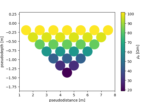
# type 2 pseudosection
fig, ax, cb = ert.pseudosection_type2('rho_a', interpolate=False, spacing=1)
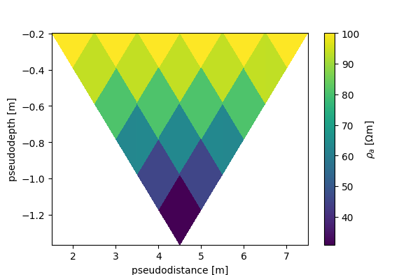
# type 2 pseudosection, interpolated
fig, ax, cb = ert.pseudosection_type2('rho_a', interpolate=True, spacing=1)
# sphinx_gallery_multi_image = "single"
<reda.containers.CR.CR object at 0x7f9766d7a560>
    a  b   m  n         r  rpha  id norrec  rdiff  rphadiff
0   1  2   4  3  5.390446 -50.0   0    nor    NaN       NaN
1   1  2   5  4  1.288918 -50.0   1    nor    NaN       NaN
2   1  2   6  5  0.436769 -50.0   2    nor    NaN       NaN
3   1  2   7  6  0.166427 -50.0   3    nor    NaN       NaN
4   1  2   8  7  0.066955 -50.0   4    nor    NaN       NaN
5   1  2   9  8  0.027893 -50.0   5    nor    NaN       NaN
6   1  2  10  9  0.012003 -50.0   6    nor    NaN       NaN
7   2  3   5  4  5.390438 -50.0   7    nor    NaN       NaN
8   2  3   6  5  1.288937 -50.0   8    nor    NaN       NaN
9   2  3   7  6  0.437061 -50.0   9    nor    NaN       NaN
10  2  3   8  7  0.166431 -50.0  10    nor    NaN       NaN
11  2  3   9  8  0.066996 -50.0  11    nor    NaN       NaN
12  2  3  10  9  0.027958 -50.0  12    nor    NaN       NaN
13  3  4   6  5  5.389588 -50.0  13    nor    NaN       NaN
14  3  4   7  6  1.289716 -50.0  14    nor    NaN       NaN
15  3  4   8  7  0.436941 -50.0  15    nor    NaN       NaN
16  3  4   9  8  0.166461 -50.0  16    nor    NaN       NaN
17  3  4  10  9  0.067026 -50.0  17    nor    NaN       NaN
18  4  5   7  6  5.397287 -50.0  18    nor    NaN       NaN
19  4  5   8  7  1.288873 -50.0  19    nor    NaN       NaN
20  4  5   9  8  0.436897 -50.0  20    nor    NaN       NaN
21  4  5  10  9  0.166363 -50.0  21    nor    NaN       NaN
22  5  6   8  7  5.390270 -50.0  22    nor    NaN       NaN
23  5  6   9  8  1.289243 -50.0  23    nor    NaN       NaN
24  5  6  10  9  0.436633 -50.0  24    nor    NaN       NaN
25  6  7   9  8  5.391080 -50.0  25    nor    NaN       NaN
26  6  7  10  9  1.287954 -50.0  26    nor    NaN       NaN
27  7  8  10  9  5.390272 -50.0  27    nor    NaN       NaN