Note
Go to the end to download the full example code.
Importing FZJ EIT40/EIT160 data
This example shows how to import data from the various versions of the EIT system developed by Zimmermann et al. 2008 (http://iopscience.iop.org/article/10.1088/0957-0233/19/9/094010/meta).
At this point we only support 3-point data, i.e., data which uses two electrodes to inject current, and then uses all electrodes to measure the resulting potential distribution against system ground. Classical four-point configurations are then computed using superposition.
Required are two files: a data file (usually eit_data_mnu0.mat and a text file (usually configs.dat containing the measurement configurations to extract.
The configs.dat file contains the four-point spreads to be imported from the measurement. This file is a text file with four columns (A, B, M, N), separated by spaces or tabs. Each line denotes one measurement:
1   2   4   3
2   3   5   6
An alternative to the config.dat file is to permute all current injection dipoles as voltage dipoles, resulting in a fully normal-reciprocal configuration set. This set can be automatically generated from the measurement data by providing a special function as the config-parameter in the import function. This is explained below.
Import reda
import reda
Initialize an sEIT container
seit = reda.sEIT()

# import the data
seit.import_eit_fzj(
    filename='data_EIT40_v_EZ-2017/eit_data_mnu0.mat',
    configfile='data_EIT40_v_EZ-2017/configs_large_dipoles_norrec.dat'
)
Constructing four-point measurements
Summary:
                a           b  ...     frequency          rpha
count  16280.0000  16280.0000  ...  16280.000000  16280.000000
mean      10.5250     30.4750  ...   1328.935406   1232.306629
std        5.8096      5.8096  ...   2885.893725   1823.550170
min        1.0000     20.0000  ...      0.100000  -3141.584482
25%        5.7500     25.7500  ...      1.000000     -9.388102
50%       10.5000     30.5000  ...     31.250000     -1.038730
75%       15.2500     35.2500  ...   1000.000000   3132.171261
max       21.0000     40.0000  ...  10000.000000   3141.580651

[8 rows x 7 columns]
an alternative would be to automatically create measurement configurations from the current injection dipoles:
from reda.importers.eit_fzj import MD_ConfigsPermutate

# initialize an sEIT container
seit_not_used = reda.sEIT()

# import the data
seit_not_used.import_eit_fzj(
    filename='data_EIT40_v_EZ-2017/eit_data_mnu0.mat',
    configfile=MD_ConfigsPermutate
)
Constructing four-point measurements
Summary:
                a           b  ...     frequency          rpha
count  16280.0000  16280.0000  ...  16280.000000  16280.000000
mean      10.5250     30.4750  ...   1328.935406    217.078193
std        5.8096      5.8096  ...   2885.893725   1129.623431
min        1.0000     20.0000  ...      0.100000  -3141.556931
25%        5.7500     25.7500  ...      1.000000    -15.614618
50%       10.5000     30.5000  ...     31.250000     -7.626176
75%       15.2500     35.2500  ...   1000.000000     -5.227314
max       21.0000     40.0000  ...  10000.000000   3141.584591

[8 rows x 7 columns]
Compute geometric factors
compute normal and reciprocal pairs note that this is usually done on import once.
quadrupoles can be directly accessed using a pandas grouper
print(seit.abmn)
quadpole_data = seit.abmn.get_group((10, 29, 15, 34))
print(quadpole_data[['a', 'b', 'm', 'n', 'frequency', 'r', 'rpha']])
<pandas.core.groupby.generic.DataFrameGroupBy object at 0x7fd3d6fb44f0>
        a   b   m   n     frequency         r        rpha
748    10  29  15  34      0.100000  7.356375   -5.205543
2228   10  29  15  34      0.314465  7.323810   -6.903037
3708   10  29  15  34      1.000000  7.282164   -7.242394
5188   10  29  15  34      3.125000  7.239073   -6.332998
6668   10  29  15  34     10.000000  7.199660  -12.081013
8148   10  29  15  34     31.250000  7.176920   -3.132819
9628   10  29  15  34    110.000000  7.170031    4.958888
11108  10  29  15  34    312.500000  7.211899    8.671063
12588  10  29  15  34   1000.000000  7.325287   -2.429873
14068  10  29  15  34   3150.000000  7.313380  -37.892727
15548  10  29  15  34  10000.000000  7.035541 -100.904824
in a similar fashion, spectra can be extracted and plotted
spec_nor, spec_rec = seit.get_spectrum(abmn=(10, 29, 15, 34))

print(type(spec_nor))
print(type(spec_rec))

with reda.CreateEnterDirectory('output_eit_fzj'):
    spec_nor.plot(filename='spectrum_10_29_15_34.pdf')

# Note that there is also the convenient script
# :py:meth:`reda.sEIT.plot_all_spectra`, which can be used to plot all spectra
# of the container into separate files, given an output directory.
<class 'reda.eis.plots.sip_response'>
<class 'reda.eis.plots.sip_response'>
filter data
seit.remove_frequencies(1e-3, 300)
seit.query('rpha < 10')
seit.query('rpha > -40')
seit.query('rho_a > 15 and rho_a < 35')
seit.query('k < 400')
Remaining frequencies:
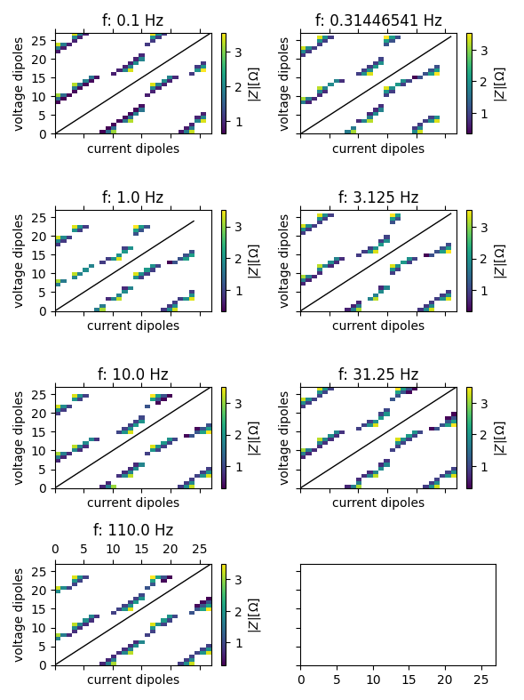
[0.1, 0.31446541, 1.0, 3.125, 10.0, 31.25, 110.0]
Plotting histograms Raw data plots (execute before applying the filters):
# import os
# import reda.plotters.histograms as redahist

# if not os.path.isdir('hists_raw'):
#     os.makedirs('hists_raw')

# # plot histograms for all frequencies
# r = redahist.plot_histograms_extra_dims(
#     seit.data, ['R', 'rpha'], ['frequency']
# )
# for f in sorted(r.keys()):
#     r[f]['all'].savefig('hists_raw/hist_raw_f_{0}.png'.format(f), dpi=300)

# if not os.path.isdir('hists_filtered'):
#     os.makedirs('hists_filtered')

# r = redahist.plot_histograms_extra_dims(
#     seit.data, ['R', 'rpha'], ['frequency']
# )

# for f in sorted(r.keys()):
#     r[f]['all'].savefig(
#         'hists_filtered/hist_filtered_f_{0}.png'.format(f), dpi=300
#     )
Now export the data to CRTomo-compatible files this context manager executes all code within the given directory
with reda.CreateEnterDirectory('output_eit_fzj'):
    import reda.exporters.crtomo as redaex
    redaex.write_files_to_directory(seit.data, 'crt_results', norrec='nor', )
Plot pseudosections of all frequencies
import reda.plotters.pseudoplots as PS
import pylab as plt

with reda.CreateEnterDirectory('output_eit_fzj'):
    g = seit.data.groupby('frequency')
    fig, axes = plt.subplots(
        4, 2,
        figsize=(15 / 2.54, 20 / 2.54),
        sharex=True, sharey=True
    )
    for ax, (key, item) in zip(axes.flat, g):
        fig, ax, cb = PS.plot_pseudosection_type1(item, ax=ax, column='r')
        ax.set_title('f: {} Hz'.format(key))
    fig.tight_layout()
    fig.savefig('pseudosections_eit40.pdf')
alternative
with reda.CreateEnterDirectory('output_eit_fzj'):
    seit.plot_pseudosections(
        column='r', filename='pseudosections_eit40_v2.pdf'
    )
Total running time of the script: (0 minutes 35.087 seconds)