Importing Syscal IP data

import reda

a hack to prevent large loading times…

# import os
# import pickle
# pfile = 'ip.pickle'
# if os.path.isfile(pfile):
#     with open(pfile, 'rb') as fid:
#         ip = pickle.load(fid)
# else:
#     ip = reda.TDIP()
#     ip.import_syscal_bin('data_syscal_ip/data_normal.bin')
#     ip.import_syscal_bin(
#       'data_syscal_ip/data_reciprocal.bin', reciprocals=48)
#     with open(pfile, 'wb') as fid:
#         pickle.dump(ip, fid)

normal loading of tdip data

ip = reda.TDIP()
# import pprofile
# profiler = pprofile.Profile()
# with profiler():
ip.import_syscal_bin('data_syscal_ip/data_normal.bin')
# profile.print_stats()
# exit()
ip.import_syscal_bin('data_syscal_ip/data_reciprocal.bin', reciprocals=48)


print(ip.data[['a', 'b', 'm', 'n', 'id', 'norrec']])

# import IPython
# IPython.embed()
# exit()

       a   b   m   n    id norrec
0      1   2   4   5   170    nor
1979   5   4   2   1   170    rec
1978   6   5   2   1   211    rec
1      1   2   5   6   211    nor
44     2   3   5   6   212    nor
...   ..  ..  ..  ..   ...    ...
986   42  43  47  48  1977    nor
988   43  44  47  48  1978    nor
991   48  47  44  43  1978    rec
990   48  47  45  44  1979    rec
989   44  45  47  48  1979    nor

[1980 rows x 6 columns]

import reda.utils.geometric_factors as geomK
K = geomK.compute_K_analytical(ip.data, spacing=0.25)
geomK.apply_K(ip.data, K)

import reda.utils.fix_sign_with_K as fixK
ip.data = fixK.fix_sign_with_K(ip.data)

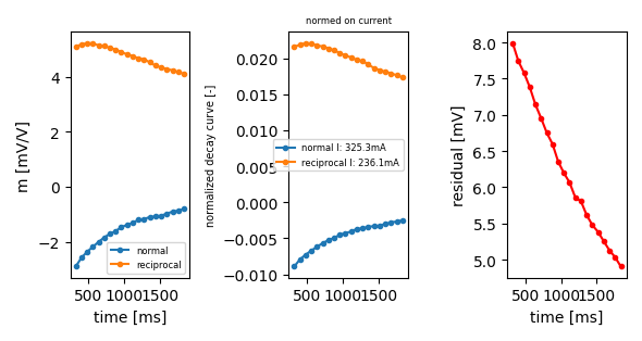
plot a decay curve by specifying the index note that no file will be saved to disk if filename parameter is not provided

ip.plot_decay_curve(filename='decay_curve.png',
                    index_nor=0, index_rec=1978, return_fig=True)

<Figure size 590.551x314.961 with 3 Axes>

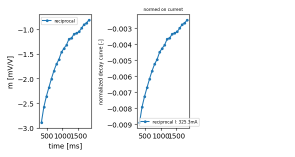
you can also specify only one index this will only return a figure object, but will not save to file:

ip.plot_decay_curve(filename='decay_curve.png',
                    index_nor=0, return_fig=True)

<Figure size 590.551x314.961 with 3 Axes>

it does not matter if you choose normal or reciprocal

ip.plot_decay_curve(index_rec=0, return_fig=True)

<Figure size 590.551x314.961 with 3 Axes>

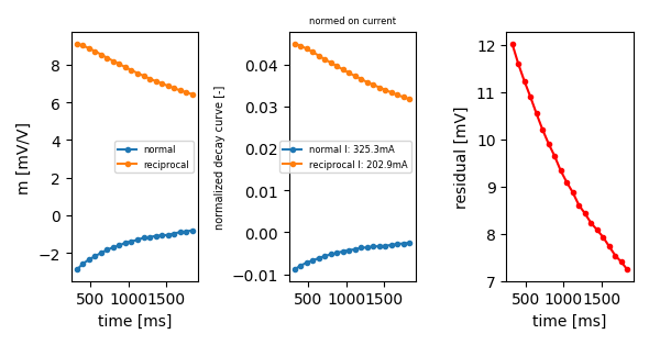
plot a decay curve by specifying the index

ip.plot_decay_curve(nr_id=170, return_fig=True)

<Figure size 590.551x314.961 with 3 Axes>

a b m n 0 1 2 4 5 1978 5 4 2 1

ip.plot_decay_curve(abmn=(1, 2, 5, 4), return_fig=True)

<Figure size 590.551x314.961 with 3 Axes>

reciprocal is also ok

ip.plot_decay_curve(abmn=(4, 5, 2, 1), return_fig=True)

<Figure size 590.551x314.961 with 3 Axes>