Visualizing ERT measurements using Pseudosections

Pseudosections are raw data representations that aim to visualize a given set of measurements in a spatial context. It is important to remember that no inversion takes place when a pseudosection is plotted, and spatial correlations should be interpreted carefully.

[TODO: 2 sentences on the basic assumption of gradually changing values]

Set up

import os

# import matplotlib.pylab as plt
import reda
ert = reda.ERT()

In this example output files are saved into subdirectories. In order to not have problems with file paths, we store the original path here

pwd = os.getcwd()

data import:

# note that you should prefer importing the binary data as the text export
# sometimes is missing some of the auxiliary data contained in the binary data.
ert.import_syscal_txt('data_syscal_ert/data_normal.txt')

# the second data set was measured in a reciprocal configuration by switching
# the 24-electrode cables on the Syscal Pro input connectors. The parameter
# "reciprocals" changes electrode notations.
ert.import_syscal_txt(
    'data_syscal_ert/data_reciprocal.txt',
    reciprocals=48
)

# compute geometrical factors using the analytical half-space equation for a
# spacing of 0.25 m
ert.compute_K_analytical(spacing=0.25)

array([-18.84955592, -18.84955592, -47.1238898 , ..., -47.1238898 ,
       -18.84955592, -18.84955592])

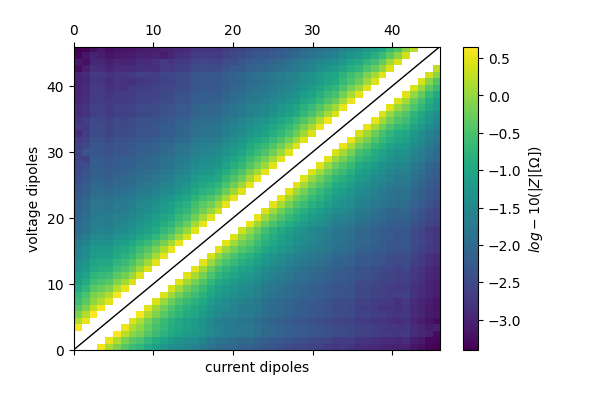
Type 1 Pseudo-sections

Type 1 pseudo-section should be mainly used for Dipole-Dipole configurations

with reda.CreateEnterDirectory('output_04'):
    ert.pseudosection_type1(
        column='r', filename='pseudosection_type1_log10_r.pdf', log10=True)

Type 2 Pseudo-sections

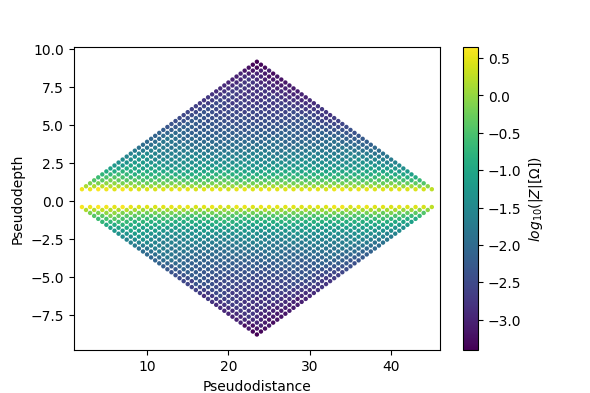
Type 2 pseudo-sections computes pseudo-locations depending on the logical electrode denotations The x-position is computed by averaging over all four a,b,m,n numbers. A heuristic tries to differentiate between Dipole-Dipole configurations and all other configurations and assigns z-positions accordingly: * Dipole-Dipole: 0.195 * abs(b-a) * The rest: max. electrode distance * 0.3

with reda.CreateEnterDirectory('output_04'):
    ert.pseudosection_type2(
        column='r', filename='pseudosection_type2_log10_r.pdf', log10=True)

Type 3 Pseudo-sections

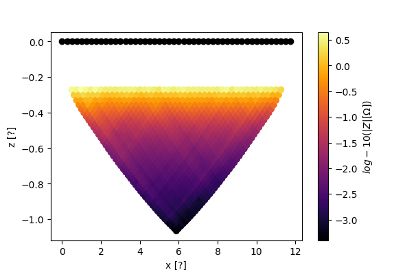
Type 3 pseudo-sections conduct a Finite-Element forward modelling, using a provided mesh, and assigns pseudo-locations to the measurements by computing center of masses for all configurations. To use this type of pseudo-section, a working CRMod installation is required

with reda.CreateEnterDirectory('output_04'):
    crmod_settings = {
        # link to file paths of elem.dat/elec.dat, CRTomo-specific mesh format
        'elem': pwd + os.sep + 'data_syscal_ert/elem.dat',
        'elec': pwd + os.sep + 'data_syscal_ert/elec.dat',
        'rho': 100,
        '2D': False,
        'sinke_node': None,
    }
    ert.pseudosection_type3(
        column='r',
        filename='pseudosection_type3_log10_r.pdf',
        log10=True,
        crmod_settings=crmod_settings,
    )

This grid was sorted using CutMcK. The nodes were resorted!
Rectangular grid found
reading sensitivities