Note
Go to the end to download the full example code.
Importing Syscal ERT data
This example is all about import data from IRIS Instruments Syscal systems. There is a variety of different options that should cover most use cases. Also, shortly introduced are the data journal, action log, filtering, and accessing data using the underlying dataframe.
import numpy as np
import matplotlib.pylab as plt
import reda
ert = reda.ERT()
data import:
# note that you should prefer importing the binary data as the text export
# sometimes is missing some of the auxiliary data contained in the binary data.
ert.import_syscal_txt('data_syscal_ert/data_normal.txt')

# the second data set was measured in a reciprocal configuration by switching
# the 24-electrode cables on the Syscal Pro input connectors. The parameter
# "reciprocals" changes electrode notations.
ert.import_syscal_txt(
    'data_syscal_ert/data_reciprocal.txt',
    reciprocals=48
)

# compute geometrical factors using the analytical half-space equation for a
# spacing of 0.25 m
ert.compute_K_analytical(spacing=0.25)
array([-18.84955592, -18.84955592, -47.1238898 , ..., -47.1238898 ,
       -18.84955592, -18.84955592], shape=(1980,))
ert.print_data_journal()
--- Data Journal Start ---
2026-05-19 07:37:40.155379
Data was imported from file  (990 data points)
Data was imported from file  (990 data points)
--- Data Journal End ---
ert.print_log()
2026-05-19 07:37:39,711 - reda.containers.BaseContainer - INFO - IRIS Syscal Pro text import
2026-05-19 07:37:39,891 - reda.containers.BaseContainer - INFO - Data sized changed from 0 to 990
2026-05-19 07:37:39,891 - reda.containers.BaseContainer - INFO - IRIS Syscal Pro text import
2026-05-19 07:37:40,150 - reda.containers.BaseContainer - INFO - Data sized changed from 990 to 1980
create some plots in a subdirectory
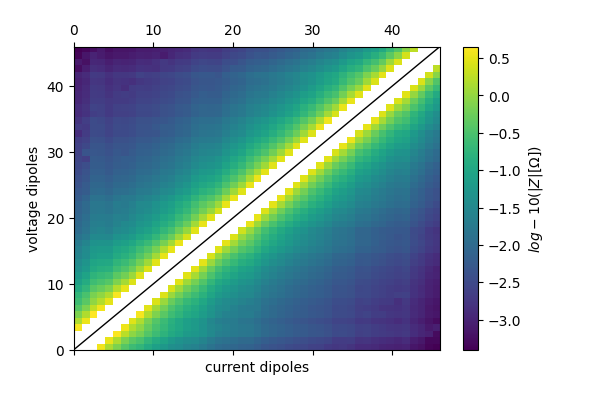
with reda.CreateEnterDirectory('plots'):
ert.pseudosection(
column='r', filename='pseudosection_log10_r.pdf', log10=True)
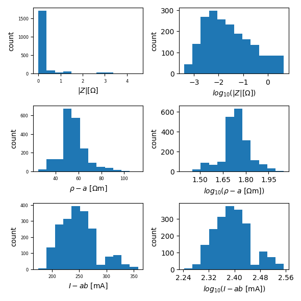
ert.histogram(['r', 'rho_a', 'Iab', ], filename='histograms.pdf')
export to various data files
with reda.CreateEnterDirectory('output_01_syscal_import'):
    ert.export_bert('data.ohm')
    ert.export_pygimli('data.pygimli')
    ert.export_crtomo('volt.dat')
The data is internally stored in a pandas.DataFrame As such, you can always use the data directly and build your custom functionality on top of REDA
print(ert.data)
       a   b   m   n      Iab  ...  norrec     rdiff          k      rho_a   sigma_a
0      1   2   5   4  325.250  ...     nor  0.248598  18.849556  73.639666  0.013580
1979   4   5   2   1  202.874  ...     rec  0.248598  18.849556  68.953711  0.014502
1      1   2   6   5  325.250  ...     nor  0.065825  47.123890  66.833629  0.014963
1978   5   6   2   1  236.119  ...     rec  0.065825  47.123890  63.731679  0.015691
1977   5   6   3   2  236.119  ...     rec  0.144387  18.849556  61.150591  0.016353
...   ..  ..  ..  ..      ...  ...     ...       ...        ...        ...       ...
992   47  48  43  42  245.897  ...     rec  0.000643  94.247780  33.816547  0.029571
991   47  48  44  43  245.897  ...     rec  0.006144  47.123890  39.687461  0.025197
988   43  44  48  47  179.834  ...     nor  0.006144  47.123890  39.976982  0.025014
990   47  48  45  44  245.897  ...     rec  0.049032  18.849556  32.889082  0.030405
989   44  45  48  47  242.947  ...     nor  0.049032  18.849556  33.813317  0.029574

[1980 rows x 13 columns]
Lets apply an arbitrary filter. Note that the change in data numbers is logged. You can use all columns defined in the data frame for more complex filters
ert.filter('r <= 0')
ert.filter('(a == 1) and Iab <= 100')
ert.print_data_journal()
--- Data Journal Start ---
2026-05-19 07:37:41.251867
Data was imported from file  (990 data points)
Data was imported from file  (990 data points)
A filter was applied with query "r <= 0". In total 0 records were removed
A filter was applied with query "(a == 1) and Iab <= 100". In total 0 records were removed
--- Data Journal End ---
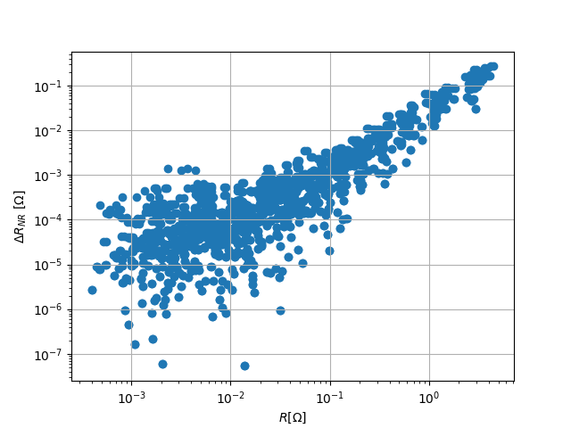
Also note that normal-reciprocal differences were directly computed.
fig, ax = plt.subplots()
ax.scatter(
    ert.data['r'],
    np.abs(ert.data['rdiff']),
)
ax.set_xlabel(r'$R [\Omega$]')
ax.set_ylabel(r'$\Delta R_{NR}~[\Omega$]')
ax.grid()
ax.set_xscale('log')
ax.set_yscale('log')
The column ‘id’ groups quadrupoles belonging to the same normal-reciprocal pair. For example, plot some of the groups
Id: 129
   a  b  m  n         r      rho_a          k      Iab
0  1  2  5  4  3.906706  73.639666  18.849556  325.250
1  4  5  2  1  3.658108  68.953711  18.849556  202.874
Id: 171
   a  b  m  n         r      rho_a         k      Iab
2  1  2  6  5  1.418254  66.833629  47.12389  325.250
3  5  6  2  1  1.352428  63.731679  47.12389  236.119
Id: 172
   a  b  m  n         r      rho_a          k      Iab
5  5  6  3  2  3.244140  61.150591  18.849556  236.119
4  2  3  6  5  3.388527  63.872224  18.849556  256.492
Id: 213
   a  b  m  n         r      rho_a         k      Iab
7  1  2  7  6  0.725030  68.332465  94.24778  325.250
6  6  7  2  1  0.717153  67.590078  94.24778  207.264
Id: 214
   a  b  m  n         r      rho_a         k      Iab
8  2  3  7  6  1.473301  69.427689  47.12389  256.492
9  6  7  3  2  1.442918  67.995919  47.12389  207.264
Id: 215
    a  b  m  n         r      rho_a          k      Iab
10  6  7  4  3  4.233244  79.794762  18.849556  207.264
11  3  4  7  6  4.500319  84.829014  18.849556  239.825
There are various ways to import Syscal data, relating to the electrode numbering:
ert1 = reda.ERT()
ert1.import_syscal_bin(
    'data_syscal_ert/02_data_normal_thinned_not_all_electrodes/data.bin',
    check_meas_nums=False,
)
print(ert1.electrode_positions)

ert2 = reda.ERT()
ert2.import_syscal_bin(
    'data_syscal_ert/02_data_normal_thinned_not_all_electrodes/data.bin',
    check_meas_nums=False,
    elecs_transform_reg_spacing_x=(1, 2.5),
)
print(ert2.electrode_positions)

ert3 = reda.ERT()
ert3.import_syscal_bin(
    'data_syscal_ert/02_data_normal_thinned_not_all_electrodes/data.bin',
    check_meas_nums=False,
    assume_regular_electrodes_x=(48, 1.0),
    # elecs_transform_reg_spacing_x=(1, 2.5),
)
print(ert3.electrode_positions)

ert_rec = reda.ERT()
ert_rec.import_syscal_bin(
    'data_syscal_ert/02_data_normal_thinned_not_all_electrodes/data.bin',
    check_meas_nums=False,
    assume_regular_electrodes_x=(48, 1.0),
    elecs_transform_reg_spacing_x=(1, 2.5),
    reciprocals=48,
)
print(ert_rec.electrode_positions)
                     x    y    z
electrode_number
1                  0.0  0.0  0.0
2                  1.0  0.0  0.0
3                  3.0  0.0  0.0
4                  4.0  0.0  0.0
5                  5.0  0.0  0.0
6                  6.0  0.0  0.0
7                  7.0  0.0  0.0
8                  8.0  0.0  0.0
9                  9.0  0.0  0.0
10                10.0  0.0  0.0
11                11.0  0.0  0.0
12                12.0  0.0  0.0
13                40.0  0.0  0.0
14                41.0  0.0  0.0
15                42.0  0.0  0.0
16                43.0  0.0  0.0
17                44.0  0.0  0.0
18                45.0  0.0  0.0
19                46.0  0.0  0.0
20                47.0  0.0  0.0
                      x    y    z
electrode_number
1                   0.0  0.0  0.0
2                   2.5  0.0  0.0
3                   7.5  0.0  0.0
4                  10.0  0.0  0.0
5                  12.5  0.0  0.0
6                  15.0  0.0  0.0
7                  17.5  0.0  0.0
8                  20.0  0.0  0.0
9                  22.5  0.0  0.0
10                 25.0  0.0  0.0
11                 27.5  0.0  0.0
12                 30.0  0.0  0.0
13                100.0  0.0  0.0
14                102.5  0.0  0.0
15                105.0  0.0  0.0
16                107.5  0.0  0.0
17                110.0  0.0  0.0
18                112.5  0.0  0.0
19                115.0  0.0  0.0
20                117.5  0.0  0.0
                     x    y    z
electrode_number
1                  0.0  0.0  0.0
2                  1.0  0.0  0.0
3                  2.0  0.0  0.0
4                  3.0  0.0  0.0
5                  4.0  0.0  0.0
6                  5.0  0.0  0.0
7                  6.0  0.0  0.0
8                  7.0  0.0  0.0
9                  8.0  0.0  0.0
10                 9.0  0.0  0.0
11                10.0  0.0  0.0
12                11.0  0.0  0.0
13                12.0  0.0  0.0
14                13.0  0.0  0.0
15                14.0  0.0  0.0
16                15.0  0.0  0.0
17                16.0  0.0  0.0
18                17.0  0.0  0.0
19                18.0  0.0  0.0
20                19.0  0.0  0.0
21                20.0  0.0  0.0
22                21.0  0.0  0.0
23                22.0  0.0  0.0
24                23.0  0.0  0.0
25                24.0  0.0  0.0
26                25.0  0.0  0.0
27                26.0  0.0  0.0
28                27.0  0.0  0.0
29                28.0  0.0  0.0
30                29.0  0.0  0.0
31                30.0  0.0  0.0
32                31.0  0.0  0.0
33                32.0  0.0  0.0
34                33.0  0.0  0.0
35                34.0  0.0  0.0
36                35.0  0.0  0.0
37                36.0  0.0  0.0
38                37.0  0.0  0.0
39                38.0  0.0  0.0
40                39.0  0.0  0.0
41                40.0  0.0  0.0
42                41.0  0.0  0.0
43                42.0  0.0  0.0
44                43.0  0.0  0.0
45                44.0  0.0  0.0
46                45.0  0.0  0.0
47                46.0  0.0  0.0
48                47.0  0.0  0.0
                      x    y    z
electrode_number
1                   0.0  0.0  0.0
2                   2.5  0.0  0.0
3                   5.0  0.0  0.0
4                   7.5  0.0  0.0
5                  10.0  0.0  0.0
6                  12.5  0.0  0.0
7                  15.0  0.0  0.0
8                  17.5  0.0  0.0
9                  20.0  0.0  0.0
10                 22.5  0.0  0.0
11                 25.0  0.0  0.0
12                 27.5  0.0  0.0
13                 30.0  0.0  0.0
14                 32.5  0.0  0.0
15                 35.0  0.0  0.0
16                 37.5  0.0  0.0
17                 40.0  0.0  0.0
18                 42.5  0.0  0.0
19                 45.0  0.0  0.0
20                 47.5  0.0  0.0
21                 50.0  0.0  0.0
22                 52.5  0.0  0.0
23                 55.0  0.0  0.0
24                 57.5  0.0  0.0
25                 60.0  0.0  0.0
26                 62.5  0.0  0.0
27                 65.0  0.0  0.0
28                 67.5  0.0  0.0
29                 70.0  0.0  0.0
30                 72.5  0.0  0.0
31                 75.0  0.0  0.0
32                 77.5  0.0  0.0
33                 80.0  0.0  0.0
34                 82.5  0.0  0.0
35                 85.0  0.0  0.0
36                 87.5  0.0  0.0
37                 90.0  0.0  0.0
38                 92.5  0.0  0.0
39                 95.0  0.0  0.0
40                 97.5  0.0  0.0
41                100.0  0.0  0.0
42                102.5  0.0  0.0
43                105.0  0.0  0.0
44                107.5  0.0  0.0
45                110.0  0.0  0.0
46                112.5  0.0  0.0
47                115.0  0.0  0.0
48                117.5  0.0  0.0
Basics plots
ert1.plot_histogram(columns='r')
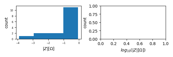
{'all': <Figure size 590.551x196.85 with 2 Axes>}