Exporting to SimPEG for ERT inversion

Example that shows how to export data to SimPEG

This example basically reuses, and simplifies, the following SimPEG tutorial:

https://simpeg.xyz/user-tutorials/inv-dcr-2d#define-and-run-the-inversion

Work in progress example!

sphinx_gallery_thumbnail_number = 4

import reda
import matplotlib as mpl
import matplotlib.pyplot as plt
import numpy as np

simpeg-specific imports

from simpeg.data import Data
from simpeg.electromagnetics.static.utils.static_utils import (
    plot_pseudosection,
)
from discretize import TreeMesh
from discretize.utils import active_from_xyz
from simpeg.electromagnetics.static.utils import (
    generate_survey_from_abmn_locations,
)
from simpeg import (
    maps,
    # data,
    data_misfit,
    regularization,
    optimization,
    inverse_problem,
    inversion,
    directives,
)

from simpeg.electromagnetics.static import resistivity as dc

mpl.use('Agg')
# import warnings
# import simpeg
# warnings.filterwarnings(
#     'ignore', simpeg.utils.solver_utils.DefaultSolverWarning
# )

import data into reda, including electrode information

data_e = reda.ERT()
data_e.import_syscal_bin('../01_ERT/data_rodderberg/20140208_01.bin')
data_e.import_electrode_positions(
    '../01_ERT/data_rodderberg/electrode_positions.dat',
)

# plot the electrode positions
# data.plot_electrode_positions_2d()

with reda.CreateEnterDirectory(‘output_01_ertinv’):

data.histogram(‘r’, log10=True, filename=’histograms_raw.pdf’)

data_e.compute_K_numerical(
    {
        'rho': 100,
        'elem': '../01_ERT/data_rodderberg/mesh_creation/g1/elem.dat',
        'elec': '../01_ERT/data_rodderberg/mesh_creation/g1/elec.dat',
    }
)
data_e.filter('rho_a <= 0')

apparent_resistivities = data_e.data['rho_a'].values

# normalized voltages, also called transfer resistances
data_volt = data_e.data['r'].values

SETTINGS
{'rho': 100, 'elem': '../01_ERT/data_rodderberg/mesh_creation/g1/elem.dat', 'elec': '../01_ERT/data_rodderberg/mesh_creation/g1/elec.dat'}

a_locs = data_e.electrode_positions.iloc[data_e.data['a'] - 1, [0, 2]].values
b_locs = data_e.electrode_positions.iloc[data_e.data['b'] - 1, [0, 2]].values
m_locs = data_e.electrode_positions.iloc[data_e.data['m'] - 1, [0, 2]].values
n_locs = data_e.electrode_positions.iloc[data_e.data['n'] - 1, [0, 2]].values

survey, out_indices = generate_survey_from_abmn_locations(
    locations_a=a_locs,
    locations_b=b_locs,
    locations_m=m_locs,
    locations_n=n_locs,
    data_type="volt",
    output_sorting=True,
)

data_object = Data(survey, dobs=data_volt)

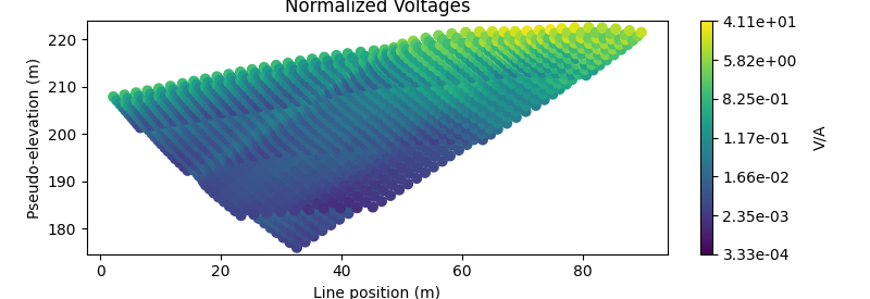
# Plot voltages pseudo-section

fig = plt.figure(figsize=(8, 2.75))
ax1 = fig.add_axes([0.1, 0.15, 0.75, 0.78])
plot_pseudosection(
    data_object,
    plot_type="scatter",
    ax=ax1,
    scale="log",
    cbar_label="V/A",
    scatter_opts={"cmap": mpl.cm.viridis},
)
ax1.set_title("Normalized Voltages")
with reda.CreateEnterDirectory('output_00_ertinv'):
    fig.savefig('pseudosection.jpg', dpi=300)

data_object.standard_deviation = 7e-5 + 0.01 * np.abs(data_object.dobs)

https://simpeg.xyz/user-tutorials/inv-dcr-2d#define-and-run-the-inversion

dh = 1  # base cell width
dom_width_x = 150.0  # domain width x
dom_width_z = 40.0  # domain width z
nbcx = 2 ** int(
    np.round(np.log(dom_width_x / dh) / np.log(2.0)))  # num. base cells x
nbcz = 2 ** int(
    np.round(np.log(dom_width_z / dh) / np.log(2.0)))  # num. base cells z

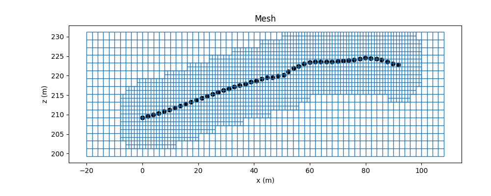
# Define the base mesh with top at z = 0 m
hx = [(dh, nbcx)]
hz = [(dh, nbcz)]
mesh = TreeMesh(
    [hx, hz],
    origin=('0', '0'),
    diagonal_balance=True,
)

topo_2d = data_e.electrode_positions[['x', 'z']].values
x_dist = np.abs(topo_2d[:, 0].max() - topo_2d[:, 0].min())

# Shift top to maximum topography
mesh.origin = mesh.origin + np.r_[-20, topo_2d[:, 1].min() - 10]

# Mesh refinement based on topography
mesh.refine_surface(
    topo_2d,
    padding_cells_by_level=[0, 0, 4, 4],
    finalize=False,
)


# Extract unique electrode locations.
unique_locations = data_object.survey.unique_electrode_locations

# Mesh refinement near electrodes.
mesh.refine_points(
    unique_locations,
    padding_cells_by_level=[8, 12, 6, 6],
    finalize=False,
)

mesh.finalize()

fig = plt.figure(figsize=(10, 4))

ax1 = fig.add_axes([0.14, 0.17, 0.8, 0.7])
mesh.plot_grid(ax=ax1, linewidth=1)
ax1.grid(False)
# ax1.set_xlim(-1500, 1500)
# ax1.set_ylim(np.max(z_topo) - 1000, np.max(z_topo))
ax1.set_title("Mesh")
ax1.set_xlabel("x (m)")
ax1.set_ylabel("z (m)")
ax1.scatter(topo_2d[:, 0], topo_2d[:, 1], color='k')

plt.show()

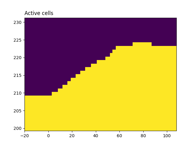
Indices of the active mesh cells from topography (e.g. cells below surface)

active_cells = active_from_xyz(mesh, topo_2d)

# number of active cells
n_active = np.sum(active_cells)

survey.drape_electrodes_on_topography(mesh, active_cells, option="top")

fig, ax = plt.subplots()
mesh.plot_image(active_cells, ax=ax)
ax.set_title('Active cells', loc='left')
fig.show()

Map model parameters to all cells

log_conductivity_map = maps.InjectActiveCells(
    mesh, active_cells, 1e-8) * maps.ExpMap(
    nP=n_active
)

# Median apparent resistivity
median_resistivity = np.median(apparent_resistivities)

# Create starting model from log-conductivity
starting_conductivity_model = np.log(
    1 / median_resistivity) * np.ones(n_active)

# Zero reference conductivity model
reference_conductivity_model = starting_conductivity_model.copy()

voltage_simulation = dc.simulation_2d.Simulation2DNodal(
    mesh,
    survey=data_object.survey,
    sigmaMap=log_conductivity_map,
    storeJ=True,
)

dmis_L2 = data_misfit.L2DataMisfit(
    simulation=voltage_simulation,
    data=data_object
)

reg_L2 = regularization.WeightedLeastSquares(
    mesh,
    active_cells=active_cells,
    alpha_s=dh**-2,
    alpha_x=1,
    alpha_y=1,
    reference_model=reference_conductivity_model,
    reference_model_in_smooth=False,
)

# WARNING: maximum number of iterations set to 2!!!!
opt_L2 = optimization.InexactGaussNewton(
    maxIter=2,
    maxIterLS=20,
    maxIterCG=20,
    tolCG=1e-3,
)

inv_prob_L2 = inverse_problem.BaseInvProblem(dmis_L2, reg_L2, opt_L2)

sensitivity_weights = directives.UpdateSensitivityWeights(
    every_iteration=True,
    threshold_value=1e-2
)

update_jacobi = directives.UpdatePreconditioner(update_every_iteration=True)
starting_beta = directives.BetaEstimate_ByEig(beta0_ratio=10)
beta_schedule = directives.BetaSchedule(coolingFactor=2.0, coolingRate=2)
target_misfit = directives.TargetMisfit(chifact=1.0)

directives_list_L2 = [
    sensitivity_weights,
    update_jacobi,
    starting_beta,
    beta_schedule,
    target_misfit,
]
# Here we combine the inverse problem and the set of directives
inv_L2 = inversion.BaseInversion(inv_prob_L2, directives_list_L2)

# Run the inversion
# recovered_model_L2 = inv_L2.run(np.log(0.01) * np.ones(n_param))
recovered_log_conductivity_model = inv_L2.run(starting_conductivity_model)

Running inversion with SimPEG v0.24.0
/home/runner/.virtualenvs/reda/lib/python3.10/site-packages/simpeg/base/pde_simulation.py:490: DefaultSolverWarning: Using the default solver: SolverLU.

If you would like to suppress this notification, add
warnings.filterwarnings('ignore', simpeg.utils.solver_utils.DefaultSolverWarning)
 to your script.
  return get_default_solver(warn=True)

                        simpeg.InvProblem is setting bfgsH0 to the inverse of the eval2Deriv.
                        ***Done using same Solver, and solver_opts as the Simulation2DNodal problem***

/home/runner/.virtualenvs/reda/lib/python3.10/site-packages/pymatsolver/wrappers.py:79: UnusedArgumentWarning: Unused keyword argument "is_symmetric" for splu.
  self.kwargs = kwargs
/home/runner/.virtualenvs/reda/lib/python3.10/site-packages/pymatsolver/wrappers.py:79: UnusedArgumentWarning: Unused keyword argument "is_positive_definite" for splu.
  self.kwargs = kwargs
/home/runner/.virtualenvs/reda/lib/python3.10/site-packages/pymatsolver/wrappers.py:81: SparseEfficiencyWarning: splu converted its input to CSC format
  self.solver = fun(self.A, **self.kwargs)
/home/runner/.virtualenvs/reda/lib/python3.10/site-packages/pymatsolver/solvers.py:415: FutureWarning: In Future pymatsolver v0.4.0, passing a vector of shape (n, 1) to the solve method will return an array with shape (n, 1), instead of always returning a flattened array. This is to be consistent with numpy.linalg.solve broadcasting.
  return self.solve(val)
model has any nan: 0
============================ Inexact Gauss Newton ============================
  #     beta     phi_d     phi_m       f      |proj(x-g)-x|  LS    Comment
-----------------------------------------------------------------------------
x0 has any nan: 0
   0  2.56e+06  2.87e+07  0.00e+00  2.87e+07    4.27e+06      0
   1  2.56e+06  1.95e+07  1.32e+00  2.29e+07    3.20e+06      0
   2  1.28e+06  1.53e+07  2.07e+00  1.80e+07    9.21e+05      0   Skip BFGS
------------------------- STOP! -------------------------
0 : |fc-fOld| = 4.9594e+06 <= tolF*(1+|f0|) = 2.8736e+06
1 : |xc-x_last| = 3.7124e+00 <= tolX*(1+|x0|) = 1.6704e+01
0 : |proj(x-g)-x|    = 9.2056e+05 <= tolG          = 1.0000e-01
0 : |proj(x-g)-x|    = 9.2056e+05 <= 1e3*eps       = 1.0000e-02
1 : maxIter   =       2    <= iter          =      2
------------------------- DONE! -------------------------

Plot the model

recovered_conductivity_L2 = np.exp(recovered_log_conductivity_model)
rec_res = 1 / recovered_conductivity_L2
plotting_map = maps.InjectActiveCells(mesh, active_cells, np.nan)
fig = plt.figure(figsize=(9, 4))

# norm = mpl.colors.Normalize(vmin=20, vmax=100)
norm = mpl.colors.LogNorm(vmin=1e0, vmax=1e3)

ax1 = fig.add_axes([0.14, 0.17, 0.68, 0.7])
mesh.plot_image(
    plotting_map * rec_res,
    ax=ax1,
    grid=False,
    # clim=[20, 100],
    pcolor_opts={
        "norm": norm,
        "cmap": mpl.cm.RdYlBu_r
    },
)
ax1.set_title('SimPEG inversion result', loc='left')
ax2 = fig.add_axes([0.84, 0.17, 0.03, 0.7])
cbar = mpl.colorbar.ColorbarBase(
    ax2,
    norm=norm,
    orientation="vertical",
    cmap=mpl.cm.RdYlBu_r,
)
with reda.CreateEnterDirectory('output_00_ertinv'):
    fig.savefig('simpeg_inversion_result.jpg', dpi=300)

print('Min/max resistivities:', rec_res.min(), rec_res.max())

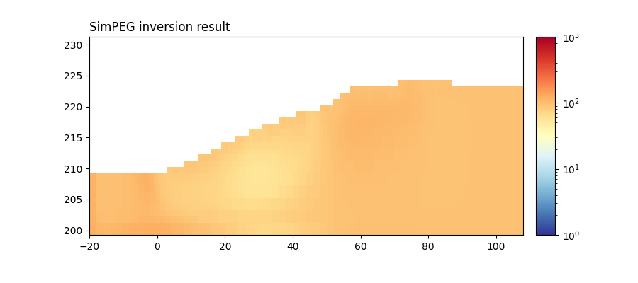
Min/max resistivities: 56.42575696453461 123.98623874271505