SIP-04 Import

The SIP04 spectral induced polarization system (Zimmermann et al., 2008 Meas. Sci. Technol. 19 105603, https://iopscience.iop.org/article/10.1088/0957-0233/19/10/105603) exports data as a .mat file and as .csv files. The ‘import_sip04’ function can load both types.

For detailed analysis of measured data, the raw time series, as measured by the system, can also be loaded.

Create the SIP container

import reda
sip = reda.SIP()

Import the SIP data

sip.import_sip04('sip_data.mat')

Import SIP04 data from .mat file
Summary:
          a     b     m     n
count  22.0  22.0  22.0  22.0
mean    1.0   4.0   2.0   3.0
std     0.0   0.0   0.0   0.0
min     1.0   4.0   2.0   3.0
25%     1.0   4.0   2.0   3.0
50%     1.0   4.0   2.0   3.0
75%     1.0   4.0   2.0   3.0
max     1.0   4.0   2.0   3.0

show the data

print(type(sip.data))
print(sip.data[['a', 'b', 'm', 'n', 'frequency', 'r', 'rpha']])

<class 'pandas.core.frame.DataFrame'>
    a  b  m  n  frequency             r       rpha
0   1  4  2  3       0.01  91710.822743 -29.362558
1   1  4  2  3       0.02  90636.299943 -28.489816
2   1  4  2  3       0.05  89244.733614 -26.907518
3   1  4  2  3       0.10  88216.019214 -26.126560
4   1  4  2  3       0.20  87199.203662 -25.008222
5   1  4  2  3       0.50  85920.509490 -22.469295
6   1  4  2  3       1.00  85104.832528 -19.333149
7   1  4  2  3       2.00  84452.492098 -15.902216
8   1  4  2  3       5.00  83819.335016 -12.312403
9   1  4  2  3      10.00  83432.605700 -10.303340
10  1  4  2  3      20.00  83104.178605  -8.858852
11  1  4  2  3      30.00  82930.728765  -8.257339
12  1  4  2  3      70.00  82606.356388  -7.006607
13  1  4  2  3     130.00  82389.613467  -6.253892
14  1  4  2  3     200.00  82254.030100  -5.743527
15  1  4  2  3     500.00  82000.383966  -4.723193
16  1  4  2  3    1000.00  81852.442931  -3.658800
17  1  4  2  3    2000.00  81744.531873  -2.586255
18  1  4  2  3    5000.00  81779.213925  -1.349227
19  1  4  2  3   10000.00  82085.647708  -3.090301
20  1  4  2  3   20000.00  82641.939514 -13.275897
21  1  4  2  3   45000.00  83175.799742 -45.989948

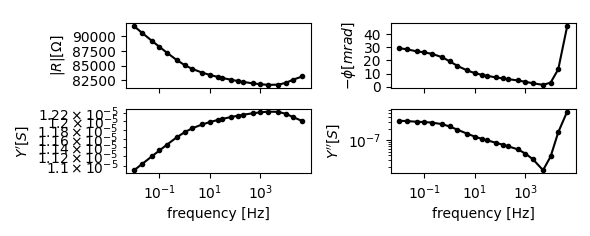
plot the spectrum

from reda.eis.plots import sip_response

spectrum = sip_response(
    frequencies=sip.data['frequency'].values,
    rcomplex=sip.data['zt'].values,
)

# note the dtype indicates that no geometric factor was applied to the data
fig = spectrum.plot(filename='spectrum.png', dtype='r', return_fig=True)

save data to ascii file

sip.export_specs_to_ascii('frequencies.dat', 'data.dat')

# optionally:
# install ccd_tools: pip install ccd_tools
# then in the command line, run:
#   ccd_single  --plot --norm 10

from reda.importers.fzj_readbin import fzj_readbin
import matplotlib.pylab as plt
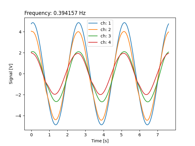
obj = fzj_readbin('data2/sip_data.bin', sip04=True)
freq_id = 15
frequency = obj.frequencies[freq_id]
times = obj.get_sample_times(frequency)
fig, ax = plt.subplots()
for channel in range(0, 4):
    ax.plot(times, obj.data[0][channel, :], label='ch: {}'.format(channel + 1))
    # break
ax.set_title(
    'Frequency: {} Hz'.format(frequency),
    loc='left',
)
ax.legend()
ax.set_ylabel('Signal [V]')
ax.set_xlabel('Time [s]')
# fig.savefig('sip04_time_series.jpg', dpi=300)

Text(0.5, 23.52222222222222, 'Time [s]')