Files and directories
config/
config.dat
config.dat contains the measurement configurations to be modelled. A
measurement configuration is defined by one or two electrodes used for current
injection and one or two electrodes used for voltage (i.e. potential
difference) measurement. By this, pole-pole, pole-dipole, and dipole-dipole,
(multiple)-gradient configurations can be realized. The format of
config.dat is explained by means of an example file:
1 2064
2 10002 40003
3 10002 50004
4 10002 60005
...
...
...
2063 300036 220016
2064 300036 230017
2065 300036 240018
- Line 1: Number of measurement configurations
- Line 2-End: Dipole configuration. The first number describes the current injection dipole using the formula \(A \cdot 10000 + B\). The second number describes the voltage dipole using the formula \(M \cdot 10000 + N\).
Pole-pole or pole-dipole configurations are realized by assigning a fictitious
electrode ‘‘0’’ (representing infinity) to the corresponding position in
config.dat. For example, the line:
10000 20000
would define a pole-pole measurement, the line
10000 20003
a pole-dipole measurement.
exe/
crt.lamnull
In order to have the option to preselect a starting value for our pareto
problem (lambda search), we introduce the lamnull_cri and lamnull_fpi
variables which can be set by the user via the file crt.lamnull.
This can contain two variables:
<lamnull_cri> (double)
<lamnull_fpi> (double)
The last one may be left empty (defaults to zero then). They are used in the
subroutine blam0 to set the lammax value.
If a complex (CRI) or DC inversion is done, the variable lamnull_cri is used.
For FPI we can use the variable lamnull_fpi, which is a NEW option.
Introduction of a separate value for the FPI is done because of two reasons:
- lam0 for the FPI changes usually dramatically if the model is changed, thus, the preselected values of lam0 for FPI may totally differ to the value for the CRI/DC.
- practical reasons for synthetic study
DEFAULT Value:
If a value of zero is choosen for each one of the lamnull_*, the program chooses:
\(\sum(diag{J^TJ})/<\text{number of parameters}> \cdot 2 /(\alpha_x + \alpha_y) * 5\)
The first is obvious, because we like to scale upon the ‘’mean’’ entries of our sensitivity matrix.
The scaling is done then to take the artificial anisotropy regularization (\(\alpha_x\) and \(\alpha_y\)) into account and last but not least multiply by five just to make sure we start right at the upper most boundary for the pareto problem.
crtomo.cfg
The crtomo.cfg file controls the inversion using CRTomo. It must exist
in the directory where CRTomo is executed. Lines starting with the
character # are treated as comments and will be removed before parsing it. All
other lines are line-number dependent. That is, each setting is identified by
its line number, not a keyword, within the crtomo.cfg file. Comment lines
do not increase the line number! The file is described by an example file:
1 2 3 4 5 6 7 8 9 10 11 12 13 14 15 16 17 18 19 20 21 22 23 24 25 26 27 28 29 30 31 32 33 34 35 36 37 38 39 40 41 42 43 44 45 46 47 48 49 50 51 52 53 54 55 56 57 58 59 60 61 62 63 64 65 66 67 68 69 70 71 72 73 74 75 76 77 78 79 80 81 82 83 84 85 86 87 88 89 90 91 92 93 94 95 96 97 98 99 100 101 102 103 104 105 106 107 108 109 110 111 112 113 114 115 116 117 118 119 120 121 122 123 124 125 126 127 128 129 130 131 132 133 134 135 136 137 138 139 140 141 142 143 144 145 146 147 148 149 150 151 152 153 154 155 156 157 158 159 160 161 162 163 164 165 166 167 168 169 170 171 172 173 174 175 176 177 178 179 180 181 182 183 184 185 186 187 188 189 190 191 192 193 194 195 196 197 198 199 200 201 202 203 204 205 206 207 208 209 210 211 212 213 214 215 216 217 218 219 220 221 222 223 224 225 226 227 228 229 230 231 232 233 234 235 236 237 238 239 240 241 242 243 244 245 246 247 248 249 250 251 252 253 254 255 256 257 258 259 260 261 262 263 264 265 266 267 268 269 270 271 272 273 274 275 276 277 278 279 280 281 282 283 284 285 286 287 288 289 290 291 292 293 294 295 296 297 298 299 300 301 302 303 304 305 306 307 308 309 310 311 312 313 314 315 316 317 318 319 320 321 322 323 324 325 326 327 328 329 330 | #############################################################
### NEW cfg file format:: ###
#############################################################
### Comment lines start with (at least one) # at the first row of a
### line!
### they are omitted during the read in of cfg file
#############################################################
#############################################################
## NOTE:
## NO FURTHER EMPTY LINES, EXCEPT THE ONES ALREADY PRESENT SHOULD BE
## GIVEN!!!
##############################################################
##############################################################
# the first line normally contains *** but may hold an integer number
# (the mega switch)
# which is evaluated bit wise and may control some things due to their Bit
# bwise setting.
# Currently implemented are:
# lsens = BTEST(mswitch,0) ! +1 write out coverage.dat (L1-norm of the
# ! sensitivities)
# (default)
# lcov1 = BTEST(mswitch,1) ! +2 write out main diagonal of
# ! posterior model covariance matrix:
# ! MCM_1=( A^T C_d^-1 A + lamda C_m^-1 )^-1
# lres = BTEST(mswitch,2) ! +4 write out main diagonal of
# resolution matrix: RES = MCM_1 * A^T C_d^-1 A
# lcov2 = BTEST(mswitch,3) ! +8 write out main diagonal of
# posterior model covariance matrix 2: MCM_2 = RES * MCM_1
# lgauss = BTEST (mswitch,4) ! +16 solve all OLS using Gauss elemination
# lelerr = BTEST (mswitch,5).OR.lelerr ! +32 uses error ellipses in the inversion,
# regardless of any previous lelerr state..
# mswitch with 2^6 is empty for now...
# lphi0 = BTEST (mswitch,7) ! +128 force negative phase
# lsytop = BTEST (mswitch,8) ! +256 enables sy top check of
# no flow boundary electrodes for enhanced beta calculation (bsytop).
# This is useful for including topographical effects
# lverb = BTEST (mswitch,10) ! +1024 Verbose output of CG iterations,
# data read in, bnachbar calculations...
#############################################################
8
#############################################################
# Path to the grid file, may contain blanks
#############################################################
../grid/elem.dat
#############################################################
# Path to the file containing electrode positions, may contain blanks
#############################################################
../grid/elec.dat
#############################################################
# Path to the measurement readings (Volts!), may contain blanks
#############################################################
../mod/volt.dat
#############################################################
# Directory name to store the inversion results.., may contain blanks
#############################################################
../inv
############################################################
# Logical switch for difference inversion (ldiff) and, if a prior model (m0) is used,
# this switch also controls whether or not to regularize against the prior..
# (internal variable lprior=T)
# leading to (m-m0)R^TR(m-m0) constraint, if no difference data are given
#########################################################################################
F
#########################################################################################
# Path to the measurement file for difference inversion, may contain blanks.
# If left empty, no data is assumed
#########################################################################################
../diff/dvolt.dat
#########################################################################################
# Path to the prior model (m0), which is also the model of the difference
# inversion which is obtained by a previous CRTomo run (dm0).
# If ldiff is false, and a valid path to a prior is given,
# the prior is copied into the starting model!!
#########################################################################################
../rho/prior.modl
#########################################################################################
# Path to the model response of m0 in case of difference inversion (ldiff=T)
# this should be empty if you have none
#########################################################################################
../diff/dvolt2.dat
#########################################################################################
# The next line usually contains nothing but *** ....
# YET, if you have a prior (or starting) model and like to add noise to it.
# You can then give a seed (integer) and a variance (float) for this.
# These numbers are useless if no prior is given..
#########################################################################################
iseed variance
#########################################################################################
# For regular grids and the old regularization you have to define the Nx (number of
# elements in x-direction)
# THIS IS NOW OBSOLETE (but can be used, though..) because the triangulation
# regularization is proofed equivalent to the old regularization for regular grids!
#
# To give it a new purpose, you can now control variogram models with it!
# The integer is read in as decimal leaving two digits (XY) with a control function
#
# _X_ Controls the covariance function and _Y_ the variogram model
#
# The variogram model has 4 modes:
# CASE (X=1) !Gaussian variogram = (1-EXP(-(3h/a)^2))
# (Ix_v = Ix_v/3 ; Iy_v = Iy_v/3: scale length are changed to match GSlib standard)
# CASE (X=2) ! Spherical variogram = ((1.5(h/a)-.5(h/a)^3),1)
# CASE (X=3) ! Power model variogram = (h/a)^omev
# in this case you can change the power model exponent, which is set to 2 as default
# CASE DEFAULT! exponential variogram = (1-EXP(-(3h/a)))
# (Ix_v = Ix_v/3 ; Iy_v = Iy_v/3)
# The default case is used if left at zero or otherwise
#
# For the covariance function there are also 4 modes implemented:
# CASE (Y=1) !Gaussian covariance = EXP(-(3h/a)^2)
# (Ix_c = Ix_c/3 ; Iy_c = Iy_c/3: scale length are changed to match GSlib standard)
# CASE (Y=2) !Spherical covariance = ((1-1.5(h/a)+.5(h/a)^3),0)
# CASE (Y=3) !Power model covariance = EXP(-va*(h/a)^omec)
# CASE (Y=4) !Lemma (still to proof!) covariance = EXP(-tfac*variogram(h))
# CASE DEFAULT!Exponential covariance = EXP(-3h/a)
# (Ix_c = Ix_c/3 ; Iy_c = Iy_c/3)
#
# The covariance model does only makes sense with a stochastical regularization!!!
#
# EXAMPLE:
# - You like to have spherical variogram but gaussian covariance set the number
# to 12
# - If you like to have a spherical variogram and a exponential covariance
# NOTE:
# The experimental variogram can be calculated (and this is default if any value
# is given) no matter which model function you state here..
#########################################################################################
0
#########################################################################################
# Previously, the next integer number was the number of cells in z- (or y)-direction
# However, the same argumentation for this number holds as for Nx.
# The new meaning for Nz is now to give a starting value for lambda:
# -value given here sets lam_0 = value
# This may be further exploited (in case you do not know and do not like the whole A^TA
# diagonal maximum to be calculated (blam0), you can leave it as -1 which will take
# lam_0 = MAX(number of data points,number of model parameters)
#########################################################################################
-1
#########################################################################################
# Now, the anisotropic regularization parameters (float) can be specified:
# alpha_x
#########################################################################################
1.0000
#########################################################################################
# alpha_z (y)
#########################################################################################
1.0000
#########################################################################################
# Next, you have to give a upper boundary for the number of iterations (int)
# NOTE:
# If it is set to zero, no inverse modelling is done, but coverages
# (resolution, variogram, etc..) may be calculated.
# This is especially useful in conjunction with a valid prior/starting model!
#########################################################################################
20
#########################################################################################
# The next (logical) switch (ldc) controls whether we invert for COMPLEX (EIT, ldc = F)
# or REAL values (ERT) (ldc = T)
#########################################################################################
F
#########################################################################################
# (logical) switch (lrobust) for robust inversion (e.g. La Breque et al 1996)
#########################################################################################
F
#########################################################################################
# Do you want a Final phase improvement (FPI) ? set (lfphai) the next logical to T
# NOTE:
# If (ldc == .FALSE. .and. lfphai == .TRUE.) lelerr = .FALSE. (error ellipses)
# This has the impact, that no error ellipses are used in FPI.
##
# However, this may be overwritten by setting mswitch = mswitch + 32 in the first line !!
#########################################################################################
T
#########################################################################################
# The next two floats determine the error model for resistance/voltage
# which is currently implemented as \delta R = A * abs(R) + B
# Thus, A gives the relative error estimate [%] and B gives the absolute error estimate.
#
# NOTE:
# The first (A) Parameter also controls whether or not to couple the (maybe COMPLEX)
# error model to any noise additions (Yes, voltages in CRTomo can be noised...)
# If A is set to -A , the whole error model is taken as noise model.
# Giving this, you may want to add an ensemble seed number, which may be crucial for
# any kind of monte carlo study, at the end of this crt-file..
# The noise is also written to the file 'crt.noisemod' which may be changed afterwards if
# you like to decouple error and noise model.
# NOTE:
# CRTomo is looking for crt.noisemod in the current directory as default.
# If it is existing or a valid file, it gives a note about this and
# trys to get a noise model from the data contained
#########################################################################################
-1.0
#########################################################################################
# Error model parameter B [Ohm]
#########################################################################################
1e-3
#########################################################################################
# Next 4 (float) numbers control the phase error model as can be found in
# Flores-Orozsco et al, 2011
# \delta \phi = A1*abs(R)^B1 + A2*abs(pha) + p0
###
# A1 [mrad/Ohm/m]
#########################################################################################
0.0
#########################################################################################
# B1 []
#########################################################################################
0.0
#########################################################################################
# A2 [%]
#########################################################################################
0.0
#########################################################################################
# p0 [mrad]
#########################################################################################
#########################################################################################
# If you use FPI, note that if P0 is set to a negative value, the phase model is set
# to a homogenous model if FPI starts, this was used by AK as default...
# the p0 is set to its positive value for error calc, if this is used (of course..)
#########################################################################################
#########################################################################################
1e-1
#########################################################################################
# Here you can decide if you want a homogenous starting model (overwritten with prior)
# logical (lrho0) for both, magnitude and phase
#########################################################################################
T
#########################################################################################
# homogenous background resistivity value for magnitude [Ohm m]
#########################################################################################
100.00
#########################################################################################
# homogenous background value for the phase [mrad]
#########################################################################################
0.000
#########################################################################################
# Some people prefer having one crt-file for many inversions.
# If you set this logical T, CRTomo tries to read in another crt-style file after
# the first inversion was done.
# This also means, that any data arrays (memory model!!) are reallocated and thus
# different grids/electrodes/measurements can be given to CRTomo...
#########################################################################################
F
#########################################################################################
# Dimensionality switch (integer) to control whether or not to have a _real_ 2D (=0)
# or a 2.5D (=1) forward solution. 2.5D assumes a 3D model space with a resistivity
# distribution that is homogeneous in the y direction.
# NOTE:
# If you like to have a true 2D (i.e. setting to 0) you have to keep in mind that
# the sink node setting (down below) has to be set.
# Also note that if 2D mode is selected the singularity removal switch may be helpful to
# reduce numerical issues.
#########################################################################################
1
#########################################################################################
# (logical) switch whether to introduce a fictitious sink node (sink is here in the sense
# of a -I electrode at some place in b by solving Ax=b with Cholesky
#########################################################################################
F
#########################################################################################
# Node number (int) of the sink node
# The chosen node should conform to the following properties:
# - not a boundary node
# - not an electrode
# - should be positioned at the center of the grid with a preferably large distance to
# all electrodes
#########################################################################################
0
#########################################################################################
# Do you like to read in some boundary potential values ? (logical)
# The boundary values are helpful for tank experiments at known voltages (i.e.
# inhomogenous Dirichlet boundaries)
#########################################################################################
F
#########################################################################################
# Path to the boundary values, blanks can be included
#########################################################################################
empty
#########################################################################################
# In some older cfg files, this would be the end of the cfg-file.
# Yet, to control regularization you can give in the next line an integer (ltri) to
# manage it:
# (=0) - Smooth regularization for regular grids only (Nx and Nz have to be correct!!)
# (=1) - Smooth triangular regularization (should be used as default and the method
# of choice
# (=2) - Smooth triangular regularization, second order (not yet implemented..)
# (=3) - Levenberg damping (i.e. C_m^-1 = lambda * I)
# (=4) - Marquardt-Levenberg damping (i.e. C_m^-1 = lambda * diag{A^T C_d^-1 A} )
# (=5) - MGS regularization (pure MGS after Zhdanov & Portniaguine):
# C_m^-1 \approx \int \frac{(\nabla m_{ij})^2}{(\nabla m_{ij})^2+\beta^2}\;dA
# (=6) - MGS with sensitivity weighted beta: = beta / f_{ij} (from Blaschek 2008)
# where f_{ij} = (1 + g(i) + g(k))^2 and g(i,k) = log_{10} coverage (m_{i,k})
# (=7) - MGS with sensitivity weighted beta (as with 6) but normalized:
# f_{ij} = ((1 + g(i) + g(k))/mean{coverage})^2
# (=8) - MGS as in 6, but here a modified version of Roland Blaschek (which I apparently
# didn't understood, but was given to me from Fred...).
# For more details please have a look into bsmatm_mod.f90 -> SUBROUTINE bsmamtmmgs
# (=9) - Same as 8, but with mean coverage normalization
# (=10) - Total variance (TV) regularization (not well tested, but I think it is BETA)
#
# NOTE:
# For MGS and TV you can specify a beta-value (0<beta<1) in this cfg!
#
# (=15) - Stochastic regularization. Here, C_m is a full matrix which needs to be
# inverted at the beginning of the inverse process. For this regu you have to
# specify a proper integral scale and covariance function (see Nx-switch).
# (>15) - not allowed
# (+32) - Fix lambda value to a given value (1 as default)
# The switch is binary tested so it is as cumulative as mswitch.
# Also it is removed after a internal logical was set true (llamf).
# The lambda value can be given in a additional line after the ltri value.
#
# NOTE:
# The order of the additional switches (fixed lambda, beta, seed) is treated like:
# - fixed lambda
# - MGS/TV beta
# - Random seed
# Each in a seperate line!
#########################################################################################
1
#########################################################################################
# The following line depends on the previous choice you made, so it may be the Random
# seed, the fixed lambda value or the MGS/TV beta.
# In case of an error (fixed format integer read!) this line is just omitted.
#
# NOTE:
# For people with cfg-files with more than one inversion run (another data set = T), the
# next line should contain the beginning of the next cfg.
#########################################################################################
lam/beta/seed
|
MGS
Todo
This section should be further explained and translated. What is MGS? This section should be translated.
Allerdings könnte die beta Bestimmung etwas zeitaufwendig sein, daher sollte MGS mehr oder weniger als post-alpha Stadium bezeichnet werden.
Unterstützt werden für diesen Integer am Ende vom crtomo.cfg-file die Zahlen 5,6 & 7. Daran anschließend kann man noch ein beta angeben, sodass das cfg file in etwa so aussieht:
------ schnip ------------
F                ! fictitious sink ?
1660             ! fictitious sink node number
F                ! boundary values ?
boundary.dat
6               ! regularization switch
0.01             ! MGS beta
- 5 ist identisch zu dem Ansatz von Zhdanov [2002], Geophysical Inverse Theory and Regularization Problems, Elsevier.
- 6 & 7 sind im Grunde die von Blaschek et al. 2008, wobei hier ein Bug von Roland gefixt wurde der mit dem update der Sensitivität und des Modells nach jedem update zu tun hatte (im Grunde wurde die Glättung nicht wieder neu berechnet was nicht ganz korrekt ist).
Note
!!! Important !!! Man kann diese Glättung aber auch fixen, wenn man das unbedingt will. Dann wird die MGS-Glättung vom Startmodell genommen, welches in der Regel ja noch keine Struktur hat. Realisiert wird dies in dem man das MGS-beta auf einen _negativen_ Wert setzt.
crmod.cfg
The file is structured as follows. It is the configuration file of CRMod.
1 ***FILES***
2 ../grid/elem.dat
3 ../grid/elec.dat
4 ../rho/rho.dat
5 ../config/config.dat
6 F
! potentials ?
7 ../mod/pot/pot.dat
8 T
! measurements ?
9 ../mod/volt.dat
10 F
! sensitivities ?
11 ../mod/sens/sens.dat
12 F ! another dataset ?
13 1 ! 2D (=0) or 2.5D (=1)
14 F ! fictitious sink ?
15 1660 ! fictitious sink node number
16 F ! boundary values ?
17 boundary.dat
18 ! optional integer switch
Line 1: Not used
Line 2: Absolute or relative path to grid (
elem.dat) fileLine 3: Absolute or relative path to electrode (
elec.dat) fileLine 4: Absolute or relative path to parameter (
rho.dat) fileLine 5: Absolute or relative path to electrode configuration (
config.dat) fileLine 6: Switch enabling (T) or disabling (F) output of potentials for the measurement configurations.
Line 7: Filename prefix for potentials. A four digit number will be appended.
Line 8: Switch to enable (T) or disable (F) output of voltages.
Line 9: Filename of voltages for all measurement configurations.
Line 10: Switch to enable (T) or disable (F) output of sensitivities.
Line 11: Filename prefix for sensitivity files.
Line 12: Set either to T in case another configuration file (Lines 1 - 18) is appended to this file (Lines 19+), or F if the configuration file consist only of 18 lines.
Line 13: Assume a 2D (0) or a 2.5D (1) subsurface
Line 14: Use a fictitious sink (T/F)
Line 15: Node number of fictitious sink
Line 16: Use user supplied boundary values (T/F)
Line 17: Filename of the boundary values
Line 18: Optional integer switch:
- +1: Enable analytical solution (lana)
- +2: Modelling with K-factor (wkfak)
- +4: Singularity removal (lsr). Please note that this option can’t be used in conjunction with the analytical solution.
decouplings.dat
Decoupling for triangular smooth cell interfaces can be done using this file. The first line contains the number of decouplings, and the subsequent lines contain one decoupling each. One decoupling consists of two integer numbers of the adjoining element cells, and one floating point value which determines the decoupling factor to be multiplied to the original regularisation. A value of 0 completely decouples the regularisation of a given interface, while a value of one does not change anything. Values larger than 1 increase the regularisation above the norm.
Example:
3
3   4   0.0
5   8   0.5
8   10  0.0
The numbering is independent of the application of the CutMcK algorithm to a given grid. Use the order of appearance in the elem.dat file for the numbering.
sens.dat
Todo
this section isn’t finished yet.
Each sens.dat contains the modelled sensitivity distribution for the
corresponding measurement configuration defined in config.dat, i.e. the
(consecutive) number in the file name corresponds to the line number in
config.dat.
The modelled sensitivity is given by \(\frac{\partial V_i}{\partial
\sigma_j} \left[\frac{V\ m}{S}\right]\), where \(V_i\) is the voltage (in
\(V\)) of the \(i\)-th measurement (assuming a unit current of 1
\(A\)), and #:math:j is the conductivity (inverse of resistivity) (in
\(S/m\)) of the \(j\)-th element (of type 8). The first line in
sens.dat contains the integrated sensitivity value \(\sum_j
\frac{\partial V_i}{\partial \sigma_j}\).
The format of sens.dat is explained by means of an example file:
   1.3385538       3140.5132
  -13.399500     -0.25000000      7.50053499E-04 -8.15268550E-07
  -7.1114998     -0.25000000      1.99041306E-03 -1.93495089E-06
  -3.6995001     -0.25000000      3.69597459E-03 -3.32863351E-06
		...
		...
		...
   38.699501      -20.442499      1.44582140E-04  5.84734394E-08
   42.111500      -20.442499      1.98332040E-04 -8.41067092E-08
   48.399502      -20.442499      2.44848023E-04 -4.05481018E-07
- Line 1:
- The first number denotes the absolute value of the sum of sensitivities (\(abs(\sum s_{ij}\)).
- The second number denotes the phase value of the sum of sensitivities in mrad (\(1000 \cdot atan(Im(\sum(s_{ij})) / Re(\sum s_{ij})))\)).
- Line 2:
- Column 1 and 2: Centered (x,z) coordinates for the element
- Column 3 and 4: Real and Imaginary parts of sensitivity
Plotting
Plotting of sensitivity files can be accomplished using the crlab_py python
library:
from crlab_py.mpl import *
import crlab_py.elem as elem
import numpy as np

if __name__ == '__main__':

elem.load_elem_file('elem.dat')
elem.load_elec_file('elec.dat')
indices = elem.load_column_file_to_elements_advanced('sens0009.dat', [2,3], False, False)
elem.plt_opt.title = ''
elem.plt_opt.cblabel = r'fill'
elem.plt_opt.reverse = True

elem.plt_opt.cbmin = -1
elem.plt_opt.cbmax = 1

elem.plot_elements_to_file('sensitivity_1.png', indices[0], scale='asinh')
elem.plot_elements_to_file('sensitivity_2.png', indices[1], scale='asinh')
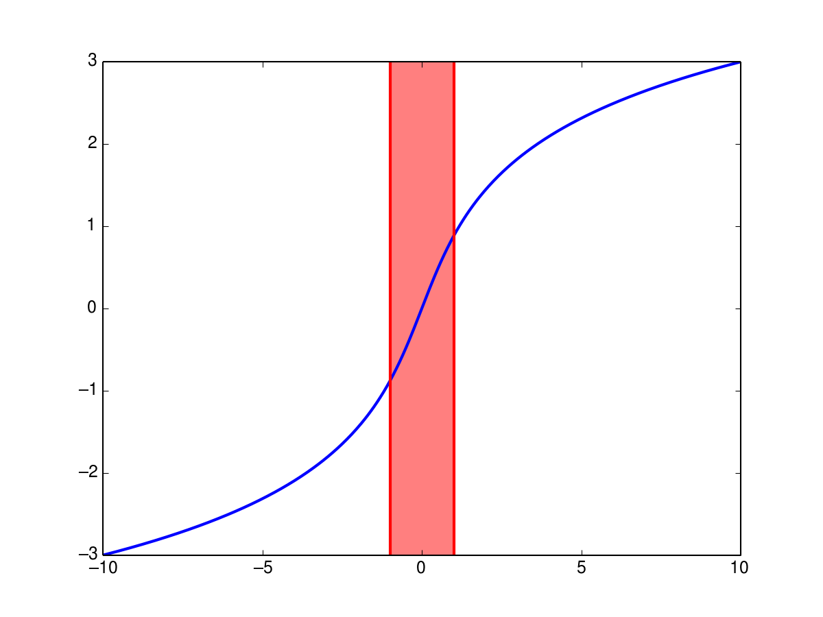
The scale-setting enables a special data transformation to plot positive and negative values over a large value range. The inverse sinus hyperbolicus shows a nearly linear behaviour between -1 and 1. Outside of this interval it shows behaviour roughly similar to the logarithm (but not the same!):
The sensitivities \(s_{ij}\) are transformed according to the formula:
The factor dyn ensures that all sensitivity values are transformed to the
value interval \(]-1,1[\). Therefore, all of them lie in the logarithmic’
range of the asinh function. All `s_{ij} values are normed to within the range
\([0,1]\) using the factor norm. The term in the arcsin-function can
thus not get larger than \(10^{\text{dyn}}\) and can be normed using the
arcsinh term in the denominator.
Warning
Always provide, or at least mention, the asinh transformation when presenting sensitivity plots. Also the normalization factor norm should be provided.
inv.elecpositions
When CRTomo is called it writes the electrode positions (as read from elem.dat
and elec.dat) to this file. The first line contains the number of (recognized)
electrodes, and each of the following lines contains two numbers: The x and z
coordinate of the corresponding electrode.
38
2.0000000000000000       -3.0000000000000000
6.0000000000000000       -3.0000000000000000
10.000000000000000       -3.0000000000000000
...
...
...
18.000000000000000       -37.000000000000000
22.000000000000000       -37.000000000000000
26.000000000000000       -37.000000000000000
inv.gstat
Created when CRTomo is called. Contains various grid statistics.
Regular grid:
Grid statistics:

Gridcells:        9360
ESP Min/Max:        0.5000    0.5000
GRID Min/Max:       0.5000   82.9247
GRID-x Min/Max:     0.5000   29.5000
GRID-y Min/Max:     0.5000   77.5000
Mean/Median/Var:        0.5000    0.5000    0.0000
Todo
Does this hold for irregular grids?
inv.lastmod
- For DC/complex inversion: Holds the (relative) path to the final iteration’s .mag file
- For FPI: Holds the (relative) path to the FPI final iteration’s .mag file
inv.lastmod_rho
Only created if FPI is used: Holds the (relative) path to the final iteration’s .mag file of the complex inversion.
grid/
elec.dat
elec.dat contains the electrode information, i.e. the numbers of nodes
where electrodes are located (the node position is determined in elec.dat). The
format of elec.dat is explained by means of an example file:
36
962
964
...
2788
2870
2952
- Line 1: Number of electrodes.
- Line 2-End: Node numbers (as defined in
elem.dat) where electrodes are located.
elem.dat
elem.dat contains all necessary information on the finite-element
discretization to be used, including the position and numbering of nodes which
constitute individual elements. The format of elem.dat is explained in the
following by means of an example file (Line numbers are prefixed in each
line):
{\tiny
\begin{verbatim}

     1	861 3 42
     2	8 800 4
     3	12 40 2
     4	11 80 2
     5	1 -7.5 0
         ...
         ...
         ...
   865	861 22.5 -12.5
   866	42 43 2 1
         ...
         ...
         ...
  1665	860 861 820 819
  1666	1 2
         ...
         ...
         ...
  1705	40 41
  1706	41 82
         ...
         ...
         ...
  1785	42 1
  1786	1
         ...
         ...
         ...
  1905	1
\end{verbatim}
}
- Line 1:
- First column: Number of nodes
- Second column: Number of element types
- Third column: Bandwidth of the resulting finite-element matrix
Line 2-4: For each element type (in this example there are three: 8 (rectangles), 11 (Mixed), 12 (Neumann)), list the following:
- First column: Element type
- Second column: Number of elements for this type
- Third column: Numnber of element this type has. Elements with 2 nodes are called degenerated
- Lines 5 - 865: Node coordinates. 3 Columns:
1 Node number: Internal Finite-Element number for this node. 2 X-coordinate 3 Z-coordinate (positive direction: upwards)
Lines 866 - 1665: Nodes of the first element type. In this case four nodes define one rectangular cell.
Lines 1666 - 1705: Nodes of second element type. In this case two nodes define a boundary condition of type 12 (Neumann).
Lines 1706 - 1785: Nodes of second element type. In this case two nodes define a boundary condition of type 11 (Mixed).
Lines 1786 - 1905: Number of the element of type 8 adjacent to the boundary elements (in the order of previous appearance).
Notes:
- Elements need to be defined counter-clockwise
- Boundary elements are defined from left to right (clockwise!)
The bandwith of the resulting finite-element matrix, the last entry in line 1 of elem.dat, is given by one plus the occurring maximal difference between the numbers of any two nodes belonging to the same element. It is thus dependent on the employed numbering of nodes.
In the present CRMod version, only elements of type 8 (quadrangular element composed of four triangular elements) and boundary elements of type 12 (homogeneous Neumann boundary condition; to be used at the Earth’s surface or at boundaries of a confined tank) or type 12 (mixed, or absorbing, boundary condition; to be used at boundaries within a half or full space) are supported.
In elem.dat, boundary elements must be listed after the normal (areal)
elements. Along the edges of elements, a linear behaviour of the electric
potential is assumed. Although elements may exhibit an irregular shape,
elements with acute angles should be avoided.
Note
New regular grids (elem.dat and elec.dat) can be created using Griev!
inv/
cjg.ctr
For each iteration, save the residuum of each Conjugate Gradient step. The
number of CG-steps can also be found in the inv.ctr file for each
iteration.
coverage.mag
L1 cumulated sensitivity (normalized)
\(S_i^{L1} = \sum_j^N \frac{|\partial V_j|}{|\partial \rho_i|}\)
2880
0.25000000000000000      -0.25000000000000000      -0.55853918225079879
0.75000000000000000      -0.25000000000000000      -0.28004078693583917
...
1.2500000000000000      -0.25000000000000000      -0.12203557213931025
1.7500000000000000      -0.25000000000000000      -0.14832386170628217
Max:   874956.88680652122
- First column: Central x-coordinate of cell
- Second column: Central z-coordinate of cell
- Third column: \(log_{10}\left( \frac{S_{ij}}{S_{ij}^{max}}\right)\) (Normalized log10 of summed sensitivities)
The last line starting with ‘Max:’ holds the maximum of the cumulated sensitivities which was used to normalize the value. As the third column is log_{10}, only negative or zero values can be expected (0-1).
coverage.mag.fpi
Contains the coverage (L1) of the sensitivties used in the FPI (thus only updating the phase component of the complex resistivity) for the final model.
The structure of the file can be found in the preceding section
(coverage.mag).
ata.diag
L2 cumulated sensitivity (normalized)
\(S_i^{L2} = \sum_j^N \frac{|\partial V_j|^2}{|\partial \rho_i|^2}\)
2880
397261824.     -0.868474960
1.72104538E+09 -0.231760025
...
2.93462502E+09   0.00000000
2.03916826E+09 -0.158099174
Max/Min:   2.93462502E+09 /   27.3748341
- First column: Diagonal entry of \(A^T C_d^{-1} A\): d_i
- Second column: \(log_{10} \left(\frac{d_i}{d_{max}}\right)\)
The last line starting with ‘Max/Min:’ holds the maximum and minimum of the cumulated sensitivities. The maximum was used to normalize the value. As the second column contains only \(log_{10}\) values only negative or zero values can be expected (i.e. values in the range between zero and one).
With \(C_d{^-1} = W_d^T W_d\); \(W_d = diag \left(\frac{1}{\epsilon_1}, \ldots, \frac{1}{\epsilon_n} \right)\)
ata_reg.diag
- First column: Diagonal entry of \(A^T C_d^{-1} A + C_m^{-1}(\lambda)\): \(d_i\)
- Second column: \(log_{10} \left(\frac{d_i}{d_{max}}\right)\)
Question: In what way are these values normalized?
cov1_m.diag and cov2_m.diag
- Cov1: \(\left[A^T C_d^{-1} A + C_m^{-1}(\lambda) \right]^{-1}\)
- Cov2: \(\left[A^T C_d^{-1} A + C_m^{-1}(\lambda) \right]^{-1} A^T C_d^{-1} A \left[A^T C_d^{-1} A + C_m^{-1}(\lambda) \right]^{-1}\)
What can I do with these files?
Both files have the format:
std err (%) | \(\delta(\sigma')\) | \(\delta(\sigma'')\)
In order to get an absolute uncertainty for a given paramter (magnitude AND phase), use the formula:
\(\delta Parameter = Parameter \cdot \frac{std err}{100}\)
For more information have a look at the ModelProbe documents D2.1.2_UBO.pdf and M2.2_UBO.pdf, which can be found in the CRTomo repository.
Examples can also be found in the examples/ subdirectory of the CRTomo repository.
res_m.diag
Stores the resolution matrix, computed from the last iteration. This file is written if the value 4 is added to the mswitch. Resolution matrix:
\(\left[A^T C_d^{-1} A + C_m^{-1}(\lambda) \right]^{-1} A^T C_d^{-1} A\)
- the first row has four columns:
- number of values (cells)
- lambda that R was computed for
- min R value
- max R value. This is the value used to normalize the data
- second to last row:
- first column linear value, NOT normalized
- second column: \(log_{10}\) value, normalized to [0, 1].
No units [1].
For further information, have a look at the CRTomo source file bmcm_mod.f90 in SUBROUTINE bres.
eps.ctr
This file consists of two parts: The first part describes the errors in
relation to the measurements (volt.dat). The second one describes the
errors for each iteration in relation to the forward solution of the current
model space.
{\tiny
\begin{verbatim}

     1	    1/eps_r  1/eps_p      1/eps      eps_r       eps_p       eps      -log(|R|)       -Phase (rad)
     2	      14.2   20000.0      14.2     0.703E-01   0.500E-04   0.703E-01  -3.553902      0.1322917E-02
		...
		...
		...
   527	       6.0   20000.0       6.0     0.167       0.500E-04   0.167       2.276732      0.3437240E-03
   528
   529	IT#      0
   530	       eps       psi      pol     Re(f(m))       Im(f(m))
   531	   0.395        2.342500    1    0.2532884       0.000000
		...
		...
		...
  1056	   0.718E-01    5.259448    1    -3.666626       0.000000
  1057
  1058	IT#      1
  1059	       eps       psi      pol     Re(f(m))       Im(f(m))
  1060	   0.395        1.881460    1    0.4353101      0.8566426E-02
		...
		...
		...
  1585	   0.718E-01    0.509647    1    -4.007404      0.5183748E-02
  1586
  1587	IT#      2
  1588	       eps       psi      pol     Re(f(m))       Im(f(m))
  1589	   0.395        1.898024    1    0.4287698      0.8681247E-02
		...
		...
		...
  2114	   0.718E-01    0.418030    1    -4.013978      0.5163230E-02
  2115
  2116	PIT#     2
  2117	       eps       psi      pol     Re(f(m))       Im(f(m))
  2118	   0.371E-02    0.491851    1    0.4287698      0.8681247E-02
		...
		...
		...
  2643	   0.305E-02    0.050550    1    -4.013978      0.5163230E-02
  2644
  2645	PIT#     3
  2646	       eps       psi      pol     Re(f(m))       Im(f(m))
  2647	   0.371E-02    0.159764    1    0.4287700      0.6262148E-02
		...
		...
		...
  3172	   0.305E-02    0.409256    1    -4.013978      0.6258056E-02
  3173
  3174	PIT#     4
  3175	       eps       psi      pol     Re(f(m))       Im(f(m))
  3176	   0.371E-02    0.160427    1    0.4287700      0.6259686E-02
		...
		...
		...
  3701	   0.305E-02    0.409742    1    -4.013978      0.6259539E-02
\end{verbatim}
}
- Line 1: Header for the raw data description. \(eps\) is the complex error which, depending on the use of the error ellipsis, is based on both magnitude and phase errors (Error ellipsis, \(eps = \sqrt{(eps_r)^2 + (eps_p)^2}\)), or only the magnitude error (no error ellipsis, \(eps = eps_r\)). datum(Re, Im) denotes the real and imaginary parts of the measurements as stored internally in CRTomo:
\(Re(datum) = -log_e(|R|)\) (Note the natural logarithm!) and \(Im(datum) = - Phase (rad)\). \(eps_r\) is the magnitue error (logarithm) and eps_p is the phase error (rad). \(eps\) is used in the complex inversion while \(eps_p\) is used in the final phase improvement.
\(eps_r\) and \(eps\) can directly be compared to \(log_e(|R|)\) and \(eps_p\) can be compared to \(Phase (rad)\).
- Lines 2 - 527: Error descriptions for each measurement.
- Line 529: Indicates the Iteration the following data describes.
- Line 530: Header for the iteration descriptions. \(eps\) is the complex error. \(psi = \frac{d_i - f_i}{\epsilon_i}\) is the error weighted residuum of the data \(d_i\) and the forward response of the current iteration \(d_i\). \(pol\) gives the polarity of the measurements, \(d\) is the forward solution, and \(f\) is the measurement.
inv.ctr
The inv.ctr file contains all information related to the inversion results.
As such it is the most important file to assess and improve inversion results.
In the following certain parts of the file will be explained:
- Lines 1 to 10 hold information regarding the specific CRTomo version that was used in the inversion.
- Lines 11 to 44 repeat the legacy parameters of the crtomo.cfg file.
- Lines 46 to 55 contain information of the grid used and the artificial noise applied to the data.
- Lines 57 to 73 show information regarding all regularization options that can be controlled.
- Lines 75 to 87 hold various options.
- Lines 89 to 101 contain fixed constants that are hardwired into the CRTomo code.
- Line 103 separates information available before the inversion from inversion regarding the inversion process.
- Line 105 contains a header which describes all columns to follow.
- Lines 107 to 174 contain information of the complex inversion.
- Lines 178 to 195 contain information of the final phase improvement.
- Line 196 indicates that the inversion finished gracefully.
{\tiny
\begin{verbatim}
1 ##
2 ## Complex Resistivity Tomography (CRTomo)
3 ##
4 ## Git-Branch master
5 ## Git-ID 334c078edcdc3b010a9cd68c07880ae845795c2f
6 ## Compiler ifort
7 ##
8 ## Created Tue-Oct-18-14:36:17-2011
9 ##
10
11 1 # mswitch
12 ../grid/elem.dat
13 ../grid/elec.dat
14 ../mod/volt.dat
15 ../inv
16 F ! difference inversion or (m - m_{prior})
17
18
19
20 ***PARAMETERS***
21 0 ! nx-switch or # cells in x-direction
22 -1 ! nz-switch or # cells in z-direction
23 1.0000 ! smoothing parameter in x-direction
24 1.0000 ! smoothing parameter in z-direction
25 20 ! max. # inversion iterations
26 F ! DC inversion ?
27 T ! robust inversion ?
28 T ! final phase improvement ?
29 5.0000 ! rel. resistance error level (%) (parameter A1 in err(R) = A1*abs(R) + A2)
30 0.10000E-03 ! min. abs. resistance error (ohm) (parameter A2 in err(R) = A1*abs(R) + A2)
31 0.0000 ! phase error model parameter A1 (mrad/ohm^B) (in err(pha) = A1*abs(R)**B + A2*abs(pha) + A3)
32 0.0000 ! phase error model parameter B (-) (in err(pha) = A1*abs(R)**B + A2*abs(pha) + A3)
33 0.0000 ! phase error model parameter A2 (%) (in err(pha) = A1*abs(R)**B + A2*abs(pha) + A3)
34 2.5000 ! phase error model parameter A3 (mrad) (in err(pha) = A1*abs(R)**B + A2*abs(pha) + A3)
35 T ! homogeneous background resistivity ?
36 40.000 ! background magnitude (ohm*m)
37 0.0000 ! background phase (mrad)
38 F ! Another dataset?
39 0 ! 2D (=0) or 2.5D (=1)
40 T ! fictitious sink ?
41 4647 ! fictitious sink node number
42 F ! boundary values ?
43 boundary.dat
44 1
45
46 ***Model stats***
47 # Model parameters 9360
48 # Data points 535
49 Add data noise ? F
50 Couple to Err. Modl? T
51 seed 1
52 Variance 0.0000
53 Add model noise ? F
54 seed 0
55 Variance 0.0000
56
57 ******** Regularization Part *********
58 Prior regualrization F
59 Regularization-switch 1
60 Regular grid smooth F
61 Triangular regu T
62 Triangular regu2 F
63 Levenberg damping F
64 Marquardt damping F
65 Minimum grad supp F
66 MGS beta/sns1 (RM) F
67 MGS beta/sns2 (RM) F
68 MGS beta/sns1 (RB) F
69 MGS beta/sns2 (RB) F
70 TV (Huber) F
71 Stochastic regu F
72 Fixed lambda? F
73 Taking easy lam_0 : 9360.000
74
75 ******** Additional output *********
76 mswitch 1
77 Read start model? F
78 Write coverage? T
79 Write MCM 1? F
80 Write resolution? F
81 Write MCM 2? F
82 Using Gauss ols? F
83 Forcing negative phase? F
84 Calculate sytop? T
85 Verbose? F
86 Error Ellipses? F
87 Restart FPI with homogenous phase? F
88
89 ***FIXED***
90 -- Sytop [m] : -39.000
91 Force negative phase ? F
92 Ratio dataset ? F
93 Min. L1 norm 1.0000
94 Min. rel. decrease of data RMS : 0.20000E-01
95 Min. steplength : 0.10000E-02
96 Min. stepsize (||\delta m||) : 0.0000
97 Min. error in relaxation : 0.10000E-03
98 Max. # relaxation iterations : 936
99 Max. # regularization steps : 30
100 Initial step factor : 0.50000
101 Final step factor : 0.90000
102
103 -------------------------------------------------------------------------------------------------------------
104
105 ID it. data RMS stepsize lambda roughn. CG-steps mag RMS pha RMS - # data L1-ratio steplength
106
107 *************************************************************************************************************
108 IT 0 7.632 7.630 3.887 0 1.13
109 *************************************************************************************************************
110 UP 1 2.874 736. 9360. 0.1551 226 1.000
111 UP 2 2.429 731. 4680. 0.3507 179 1.000
112 UP 3 2.044 726. 2569. 0.6208 143 1.000
113 UP 4 1.762 723. 1553. 0.9112 117 1.000
114 UP 5 1.573 723. 1020. 1.183 100 1.000
115 UP 6 1.448 725. 713.1 1.424 89 1.000
116 UP 7 1.363 726. 522.3 1.637 80 1.000
117 UP 8 1.302 728. 395.7 1.833 73 1.000
118 UP 9 1.258 730. 307.4 2.016 67 1.000
119 UP 10 1.223 731. 243.5 2.194 60 1.000
120 UP 11 1.196 733. 195.9 2.368 55 1.000
121 UP 12 1.174 735. 159.6 2.543 51 1.000
122 UP 13 1.155 735. 131.3 2.732 45 1.000
123 UP 14 1.139 734. 109.1 2.932 39 1.000
124 UP 15 1.126 735. 91.30 3.123 36 1.000
125 UP 16 1.115 736. 76.90 3.321 33 1.000
126 UP 17 1.105 737. 65.12 3.543 30 1.000
127 UP 18 1.095 738. 55.43 3.786 28 1.000
128 UP 19 1.087 737. 47.42 4.049 25 1.000
129 UP 20 1.078 737. 40.74 4.324 23 1.000
130 UP 21 1.071 736. 35.15 4.639 21 1.000
131 UP 22 1.064 736. 30.45 4.973 20 1.000
132 UP 23 1.058 736. 26.48 5.331 19 1.000
133 UP 24 1.052 734. 23.10 5.715 18 1.000
134 UP 25 1.047 736. 20.21 6.091 18 1.000
135 UP 26 1.042 737. 17.73 6.491 18 1.000
136 UP 27 1.037 737. 15.59 6.913 18 1.000
137 UP 28 1.030 735. 13.76 7.422 17 1.000
138 UP 29 1.026 736. 12.18 7.897 17 1.000
139 UP 30 1.023 737. 10.80 8.405 17 1.000
140 UP 31 3.409 368. 12.18 1.974 17 0.500
141 *************************************************************************************************************
142 IT 1 1.026 736.3 12.18 7.897 17 1.235 0.9566 0 1.23 1.000
143 *************************************************************************************************************
144 UP 0 0.5746 22.2 12.18 6.673 43 1.000
145 UP 1 0.5989 22.8 18.42 5.641 46 1.000
146 UP 2 0.6257 24.6 27.23 4.841 46 1.000
147 UP 3 0.6546 27.7 39.28 4.211 51 1.000
148 UP 4 0.6850 31.5 55.25 3.718 54 1.000
149 UP 5 0.7160 35.8 75.79 3.333 56 1.000
150 UP 6 0.7479 40.5 101.4 3.023 57 1.000
151 UP 7 0.7807 45.3 132.5 2.771 58 1.000
152 UP 8 0.8144 50.2 169.0 2.560 59 1.000
153 UP 9 0.8494 55.2 210.5 2.379 61 1.000
154 UP 10 0.8853 60.1 256.1 2.222 63 1.000
155 UP 11 0.9212 64.9 304.5 2.087 66 1.000
156 UP 12 0.9564 69.4 354.2 1.970 67 1.000
157 UP 13 0.9899 73.5 403.4 1.871 68 1.000
158 UP 14 1.021 77.3 450.8 1.787 69 1.000
159 UP 15 0.7534 36.8 403.4 3.787 68 0.500
160 *************************************************************************************************************
161 IT 2 0.6577 3.546 403.4 7.405 68 1.238 0.9554 0 0.048
162 *************************************************************************************************************
163 UP 0 0.9914 66.8 403.4 1.866 68 1.000
164 UP 1 1.022 70.3 450.4 1.783 69 1.000
165 UP 2 0.7629 33.4 403.4 3.640 68 0.500
166 *************************************************************************************************************
167 IT 3 0.9914 66.77 403.4 1.866 68 1.528 0.9726 0 1.000
168 *************************************************************************************************************
169 UP 0 1.008 0.152 403.4 1.812 69 1.000
170 UP 1 0.9788 0.201 361.5 1.893 78 1.000
171 UP 2 0.9994 0.761E-01 403.4 1.837 69 0.500
172 *************************************************************************************************************
173 IT 4 1.000 0.8132E-01 403.4 1.835 69 1.536 0.9723 0 0.534
174 *************************************************************************************************************
175
176 -----------------------------------------------------------------------------------------------------------------
177
178 *************************************************************************************************************
179 PIT 4 0.9723 1.536 0.9723 0
180 *************************************************************************************************************
181 PUP 1 0.9305 0.798E-02 9360. 0.1051E-02 26 1.000
182 PUP 2 0.9263 0.144E-01 4680. 0.1684E-02 30 1.000
183 PUP 3 0.9305 0.798E-02 9360. 0.1051E-02 26 1.000
184 PUP 4 0.9348 0.438E-02 0.1808E+05 0.7200E-03 25 1.000
185 PUP 5 0.9391 0.241E-02 0.3373E+05 0.5406E-03 28 1.000
186 PUP 6 0.9437 0.134E-02 0.6071E+05 0.4388E-03 32 1.000
187 PUP 7 0.9489 0.774E-03 0.1053E+06 0.3719E-03 42 1.000
188 PUP 8 0.9560 0.526E-03 0.1749E+06 0.3192E-03 50 1.000
189 PUP 9 0.9656 0.587E-03 0.2746E+06 0.2747E-03 62 1.000
190 PUP 10 0.9772 0.952E-03 0.3992E+06 0.2385E-03 70 1.000
191 PUP 11 0.9888 0.151E-02 0.5297E+06 0.2118E-03 74 1.000
192 PUP 12 0.9985 0.207E-02 0.6415E+06 0.1943E-03 83 1.000
193 *************************************************************************************************************
194 PIT 5 0.9888 0.1509E-02 0.5297E+06 0.2118E-03 74 1.536 0.9888 0 1.000
195 *************************************************************************************************************
196 ***finished***
\end{verbatim}
}
.modl files
The first row contains the number of grid cells (conductivities). Starting with the second row, the magnitude (in \(\Omega m\)) and the phase (in \(mrad\)) are displayed for each grid cell.
.mag files
The first row again contains the number of grid cells along with the normalized magnitude or phase misfit for the current inversion iteration. The following rows contain the x and z centroid coordinates and the magnitude (in \(\Omega m\)) or phase (in \(mrad\)) value for the corresponding cell.
\(log_{10}(\rho) (\Omega m)\) \(\phi (mrad)\)
.pha files
Structure is similar to the .mag files, except that the third columns contains the element phase values in mrad.
run.ctr
Provides an overview of the inversion process. Due to the adaption to screen output, this file look somewhat garbled when viewed in a text editor.
If the inversion finished sucessfully, the used CPU time will be saved to the file (grep "\^CPU" run.ctr)
voltXX.dat
voltXX.dat contains the modelled resistances and phases for all measurement configurations for iteration XX.
Line 1: number of measurement configurations
Line 2-End: Column 1: current injection electrode pair
(CRTomo format, as defined in config.dat)
Column 2: potential reading electrode pair
(CRTomo format, as defined in config.dat)
Column 3: resistance value in Ohm
Column 4: phase value in mrad
mod/
crt-files/volt.dat
volt.dat contains the modeled or measured resistances (not resistivities) for all measurement
configurations defined in config.dat. Multiple input formats are currently
recognized. The input formats are partially determined by external switches and
partially by certain key structures in the files themselfs:
External switches:
- DC or complex inversion/fpi (ldc)
Key structures:
- individual errors (lindiv - determined from the first line of the file itself)
- there are two basic file formats recognized, the “CRTomo standard” and the “industry standard”.
The format of volt.dat is explained by means of example files:
DC/Complex/FPI case, CRTomo standard:
3
10002 40003 4.3 -0.1
20003 50004 2.3 -0.2
30004 60005 9.2 -0.6
- Line 1: number of measurement configurations (here: 3)
- Line 2-End:
- Column 1: current injection electrode pair (CRTomo format, as defined in config.dat)
- Column 2: potential reading electrode pair (CRTomo format, as defined in config.dat)
- Column 3: resistance value in \(\Omega\) (CRTomo uses a current of 1 A, thus this value can also be interpreted as a voltage!)
- Column 4: phase value (\(\varphi\)) in mrad
DC case individual errors:
3 T
10002 40003 4.3 0.43
20003 50004 2.3 0.23
30004 60005 9.2 0.92
1
- Line 1 contains the number of measurements, plus the activation switch for the individual errors.
- Lines 2-(End-1):
- Column 1: current injection electrode pair (CRTomo format, as defined in config.dat)
- Column 2: potential reading electrode pair (CRTomo format, as defined in config.dat)
- Column 3: resistance value in \(\Omega\) (CRTomo uses a current of 1 A, thus this value can also be interpreted as a voltage!)
- Column 4: Normalized individual error (see last line)
- Last line: Square root of the normalization factor of individual errors: \(\sqrt{\Delta R_{norm}}\)
Each individual error is computed using the value in column 4, multiplied with the square of the normalization factor: \(\Delta R_i = \Delta R_{norm} * R_i\). Also note that the input here is always linear, despite the inversion being formulated as log(R).
Complex/FPI case:
3 T
10002 40003 4.3 -5 0.43 0.05
20003 50004 2.3 -10 0.23 0.1
30004 60005 9.2 -200 0.92 2
1 1
- Line 1 contains the number of measurements, plus the activation switch for the individual errors.
- Lines 2-(End-1):
- Column 1: current injection electrode pair (CRTomo format, as defined in config.dat)
- Column 2: potential reading electrode pair (CRTomo format, as defined in config.dat)
- Column 3: resistance value in \(\Omega\) (CRTomo uses a current of 1 A, thus this value can also be interpreted as a voltage!)
- Column 4: phase values [mrad]
- Column 5: Normalized individual magnitude error (see last line)
- Column 6: Normalized individual phase error (see last line)
- Last line: Square root of the normalization factors of individual errors: \(\sqrt{\Delta R_{norm}} \sqrt{\Delta \varphi_{norm}}\)
pot/pot.dat
Each pot.dat contains the modelled potential distribution for the corresponding
current injection configuration defined in config.dat (assuming a unit current
of 1 \(A\)), i.e., the (consecutive) number in the file name corresponds to
the line number (+1) in config.dat. The potential values of the individual
elements are listed as determined in elem.dat.
- Line 1-End:
- Column 1: x coordinate in m
- Column 2: z coordinate in m
- Column 3: potential in V
- column 4: phase in mrad
rho/
rho.dat
rho.dat contains the resistivity distribution, i.e. the resistivity values
of the individual elements determined in elem.dat. The format of rho.dat is
explained by means of an example file:
2296                   2296 elements (of type 8)
100.000000    -5       resistivity and phase of 1st element (in m)
100.000000    -10      .
100.000000    -13.4    .
.             .
.             .
.             .
99.999756    0        .
99.999893    0        .
99.999954    0        resistivity and phase of 2296th element (in m)
- Line 1: number of elements (of type 8)
- Line 2-End:
- Column 1: resistivity in Ohmm
- Column 2: phase in mrad